Samuel Arellano, Daniel Clark, Dhyan Shah, Chandler Vaughn

2020-05-19

1 Abstract

Over the past 30 years, Real-Time Location Systems (RTLS) have become the standard for enterprises and consumers to connect to their loved ones, meet business goals, and find their way home. One place where RTLS is gaining further application is its use in helping keep students connected across college campuses. In this paper, we present how RTLS access points within a college campus building can locate handheld connected devices (such as laptops or cell phones). Underlying this methodology is the understanding of how the signal strength of a device behaves at various distances, angles and even through walls which we demonstrate in a practical application. Integral to this is testing of several machine learning clustering models that will be used to predict and identify the location of these devices using the Sum of Squared Errors as the evaluation criteria. Using Weighted and Unweighted K-Nearest Neighbors methods, we demonstrated that you can significantly increase the predictability of device location if you are able to use a combination of “co” and “cd” access points. These findings can have practical application in optimized management of resource usage and in providing elasticity to the bandwidth an enterprise uses based on the location of devices loading an access point, which can offer cost benefits.

2 Introduction

With the advent of Wi-Fi and local area networks, devices like Real-Time Location Systems (RTLS) can be leveraged for location positioning of an object in a specified area in real time. This is made possible by way of a continuous communication and feedback between a tag attached to the object being tracked and reader or array of readers. Examples of RTLS include Infrared, Bluetooth, Cellular, and Radio Frequency Identification (RFID). To operate RTLS, a scanning device is required to locate an object (such as a cell phone or laptop) based on the angle and coordinates of the object being tracked. You can use multiple scanning devices to triangulate the exact location of the object using the combination of angles in which the signal is triggering the respective receivers. Utilizing a series of wireless network signals in an office building, we will be able to detect the exact location of various objects in real time using different combinations of network devices. Here, we can perform an unweighted and weighted k-nearest neighbors (k-NN) analysis to predict the location of the unknown Online data using the Offline training data. To go further, we will be seeing if we can better predict the location of the online data using different combinations of the network device mac addresses available.

3 Literature Review

The code and methodology used for this evaluation comes primarily from Data Science in R: A Case Studies Approach to Computational Reasoning and Problem Solving by Deborah Nolan of the University of California, Berkeley and Duncan Temple Lang of the University of California, Davis. The application of the code and methodoogy were further examined and proved to be sound by Southern Methodist University, as incorporated into the lectures given by Adjunct Lecturer Bradley Blanchard as part of the university’s Quantifying The World course.

4 Method

The k-nearest neighbors method is a non-parametric classification method. Unlike parametric methods, like logistic regression, which learn the parameters through training, k-nearest neighbors uses a user defined tuning parameter k to determine how the model will be trained. The k-nearest neighbors model uses k neighbors to estimate the probability of each class g as the proportion of the k neighbors of x with that class, g.

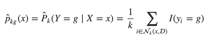
The unknown x is then assigned the class with the highest estimated probability. The k nearest neighbors are determined by a measure of distance like Euclidean distance or Manhattan distance. In unweighted models classification of x is determined the simple plurality of neighbors, but in weighted models the distances of the k neighbors will have a bearing on the classification of x.

Using the k tuning parameter, we will estimate the online device locations by assigning them with the location of k devices with the closest signal strength. We will measure the closeness in terms of signal strength of our training observations and test prediction using a Euclidean distance metric. Once we have all these measurements, we will measure the overall performance of our model by an aggregate sum of squared errors metric.

We will test are two types of k-NN algorithms: weighted and unweighted. In the case of the unweighted, the k nearest neighbors are assigned equal weight in estimating the location of the device in question. The location of the test device is simply an arithmetic average of the (x,y coordinates) of the closest nearest neighbor device. For the weighted average algorithm, the k nearest neighbors are each assigned weights that are equal to the reciprocal of their distance to the test device in terms of signal strength. Therefore, training observations with closer signal strength distances are given greater weight in estimating the location of the test observation.

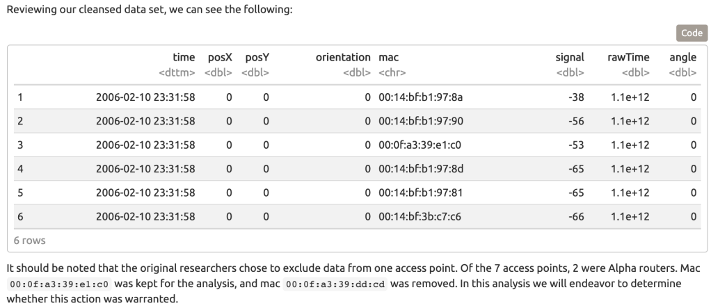
As a baseline, we will first do a search for an optimal model excluding 00:0f:a3:39:dd:cd. This will align with the original research methods of the reference case study and provide an initial set of results to compare subsequent models against.

To complete this analysis, We employed the following steps.

1. Data Cleansing
2. Exploratory Data Analysis
3. Signal Strength Analysis
4. kNN modeling
   1. Unweighted kNN
   2. Weighted kNN
5. Comparing kNN approaches

5 Data

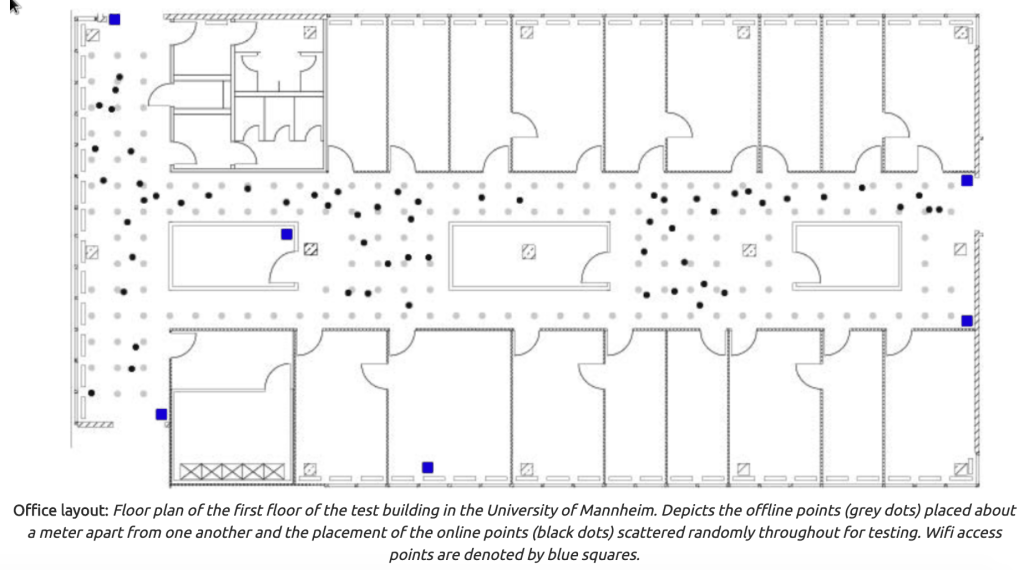
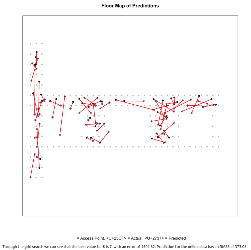
For this project, we will be leveraging two separate datasets for our analysis. One of which is a reference set named offline which contains signal strength measurements from a hand-held device on a gridwork of 166 different points, all of which were spaced 1 meter apart. This gridwork is located in the hallways of a one floor building at the University of Mannheim. The other dataset is titled online which we will be using for testing our k-NN model to predict the location of an unknown device. The online dataset includes 60 different locations chosen at random with 110 signals measured from each point by six 6 wireless access points. In figure 1.1 below, you can see a map of the online test locations (black dots) overlaid with the offline training locations (grey dots). Both datasets contain the same features and will require the same procedures for cleaning.Code

5.1 Data Description

Code

• t: Time stamp (Milliseconds) since 12:00am, January 1, 1970
• Id: router MAC address
• Pos: Router location
• Degree: Orientation of scanning device carried by the researcher, measured in Degrees
• MAC: MAC address of either the router, or scanning device, combined with corresponding values for signal strength (dBm), the mode in which it was operating(adhoc scanner = 1, access router = 3), and its corresponding channel frequency.
• Signal: Received Signal Strength in DbM

5.2 Data Formatting

The first cleaning method we will employ will be to break up the position variable into separate variables which we can use to triangulate the location. In our raw dataset, we have position values for latitude, longitude and elevation separated by commas, which we will convert into PosX, PosY and PosZ. Upon further cleaning, we were able to determine that there was only one unique value for PosZ at 0 (which made sense considering the experiment took place in a one story building), we had the liberty to drop the variable. Additionally, running a procedure to check on the number of unique variables in the ScanMac column yielded only a single unique value, so we can drop that one as well.

In our documentation, we found that our type of device was mixed between the values 1 and 3, which we may want to clarify more. Reviewing our documentation, we will only want to focus on fixed access points (value=3) as that is more relevant to our study of predicting device locations using a fixed set of receivers. So, moving further, we will remove the adhoc instances in our dataset.

The Time measurement is something that we will want to make an adjustment to so that we can more easily analyze in the future. As mentioned prior, the time data is based on the number of milliseconds from a specific date (which could possibly be arbitrary), so we can change to a Year-Month-Day-Time format. But first, we can divide the number of milliseconds to seconds. This leaves us with the following features that we will use across our offline and online data. Additionally, we will remove the channel feature since it is strictly a character code that contains redundant identifiers of Mac Address, signal strength, frequency and mode that may play an unfair role in our predictive modeling.

According to our documentation, we should have only 8 values for orientation. We also simplify our measurement of the reader orientation and round these measurements to the nearest 45 degree angle. The resolution of the existing data is less important, thus we can safely assume that 45 degree increments is sufficient, and this will provide some relief in terms of computational effort.

We will look at the orientation column of our dataset, we can see that we have a wide variety of angles available in clusters around the expected angles (such as 179 or 181) as shown in figure 2.1. Since we are going to focus on measure signal strength at 8 orientations in 45-degree increments, we will round each of our orientations to the nearest 45 degree increment. Additionally, we will try to map values close to 360 so that they line up back to zero.

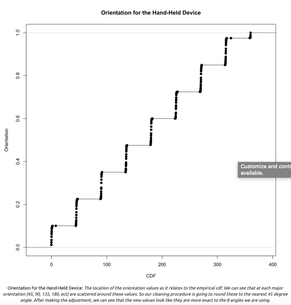
Orientation for the Hand-Held Device: The location of the orientation values as it relates to the empirical cdf. We can see that at each major orientation (45, 90, 135, 180, ect) are scattered around these values. So our cleaning procedure is going to round these to the nearest 45 degree angle. After making the adjustment, we can see that the new values look like they are more exact to the 8 angles we are using.

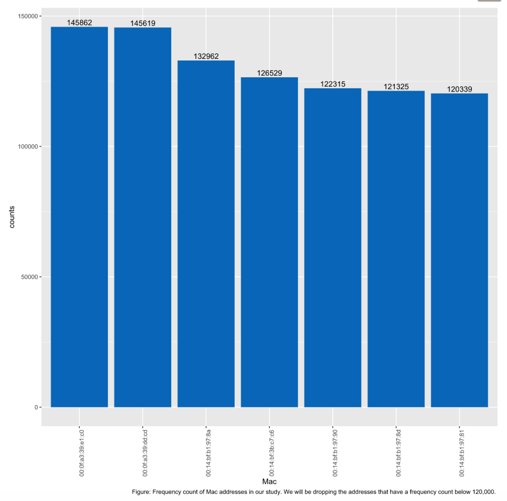
The last cleaning procedure we will follow is to review the frequency of the mac addresses in place for our models. Since the documentation mentioned that the mac addresses ending in c5, a9, fc, 10, and 4b were either not on the correct floor, or were not turned on the whole time, we have dropped these addresses so that we are only working with the remaining 7 addresses that have a frequency of over 120,000 observations.

6 RTLS Analysis

Approaching this problem strategically, we chose to analyze the received signal strength utilizing a K Nearest Neighbors approach. We first analyze the data excluding mac 00:0f:a3:39:dd:cd as definde by the original researchers. Then analyze the same data set including mac 00:0f:a3:39:dd:cd and excluding mac 00:0f:a3:39:e1:c0. Then, finally, we analyze the full data set including all access points.

6.1 Exploratory Data Analysis

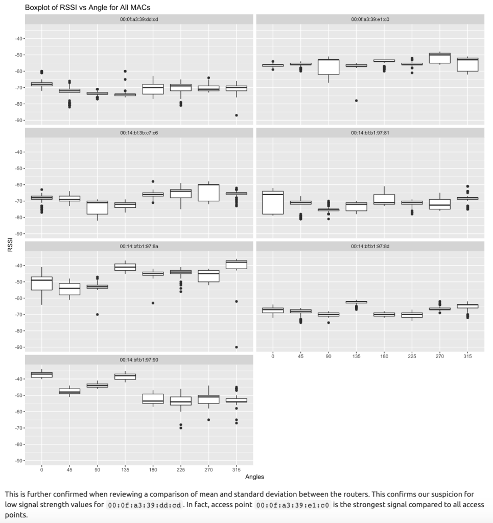
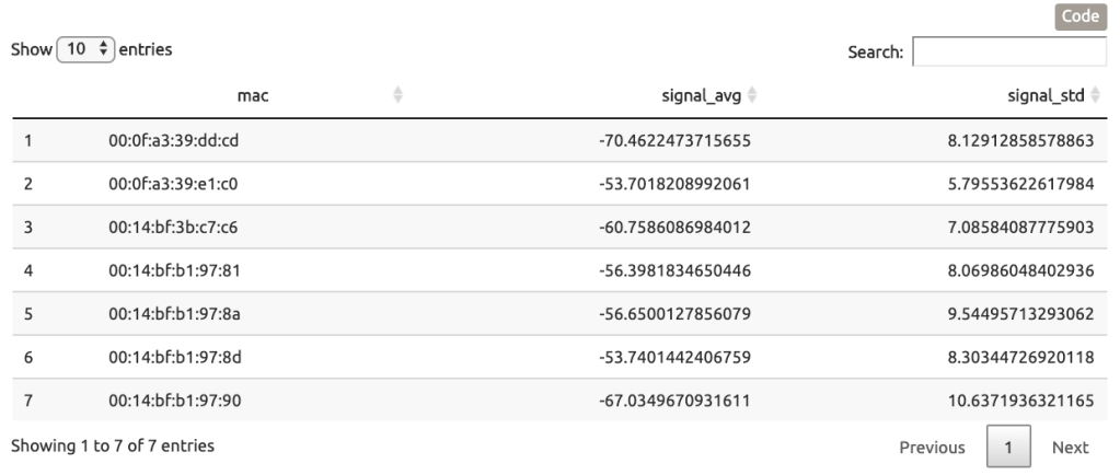
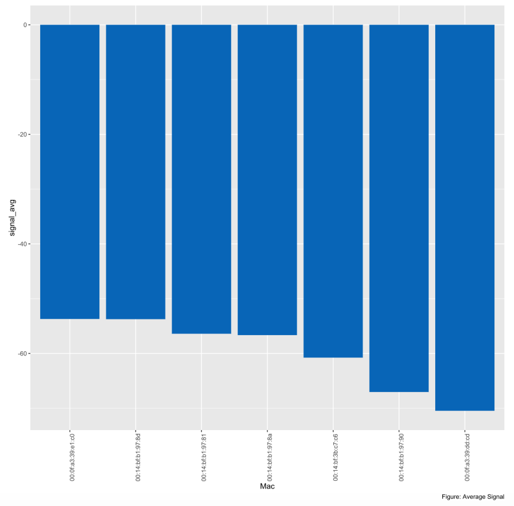
Signal Strength by Angle Given that the orientation of the signal receiving device is an important characterstic these data, we quickly review signal versus orientation angle. From these plots it becomes clear that the signal from 00:0f:a3:39:dd:cd is weak as compared to 00:0f:a3:39:e1:c0, and contains numerous outliers in the data.

6.2 Modeling: K Nearest Neighbors

In our analysis, we will use a non-parametric machine learning technique called K-Nearest_Neighbors (k-NN) to predict the position of our devices in our online dataset. For our number of neighbors we ultimately choose, we will estimate these device locations by assigning them with the location of k devices with the closest signal strenth. We will measure the closeness in terms of signal strength of our training observation and test prediction using a Euclidean metric. Once we have all these measurements, we will measure the overall performance of our model by an aggregate sum of square errors metric.

There are two types of k-NN algorithms: weighted and unweighted. In the case of the unweighted, the k nearest neighbors are assigned equal weight in estimating the location of the device in quesiton. The location of the test device is simply an arithmetic average of the (x,y coordinates) of the closest nearest neighbor device. In regards to the Weighted average, the k nearest neighbors are assigned weights that are equal to the reciprocal of its distance to the test device in terms of the signal strength. Therefore, training observations with closer signal strength distances are given greater weight in estimating the location of the test observation.

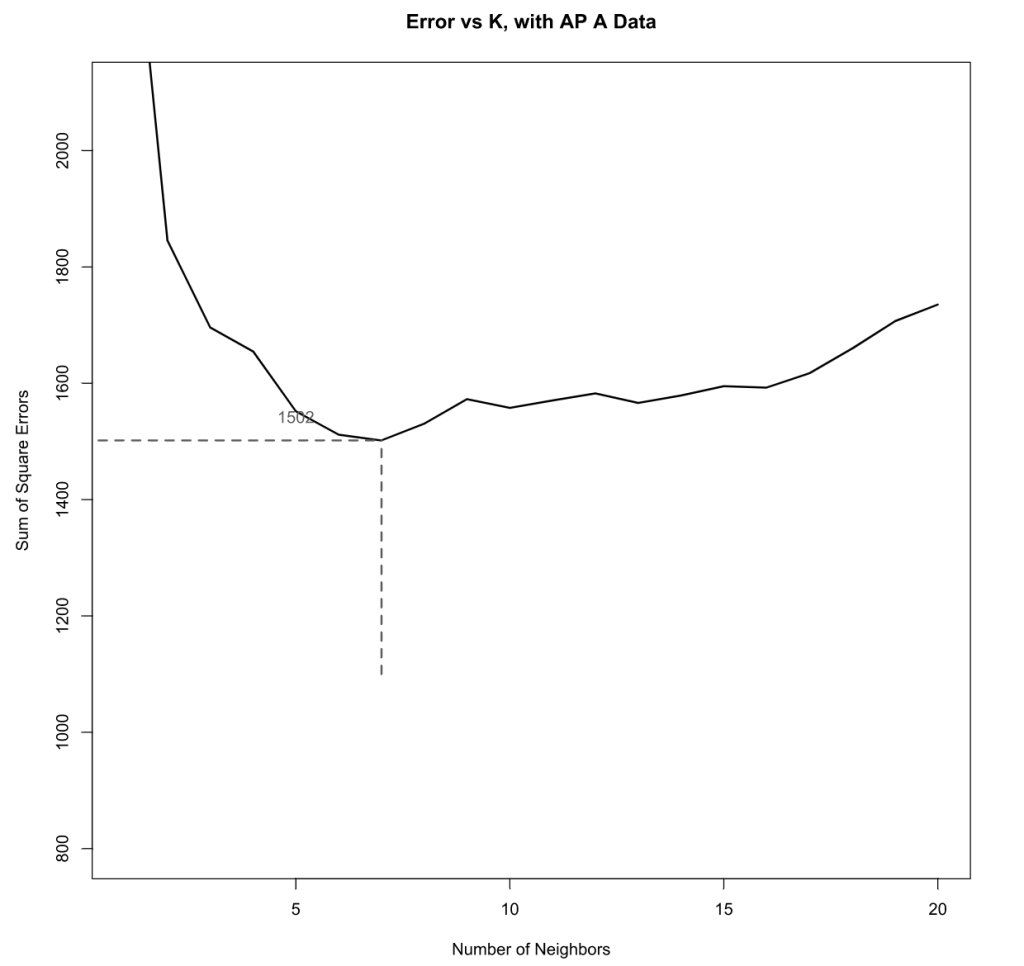
(excluding 00:0f:a3:39:dd:cd) We will first do a search for an optimal model excluding 00:0f:a3:39:dd:cd. This can serve as a baseline model to measure against since it will align with the original research methods.

Repeating the K-Nearest Neighbors Algorithm for all 6 combinations leaves us the following:

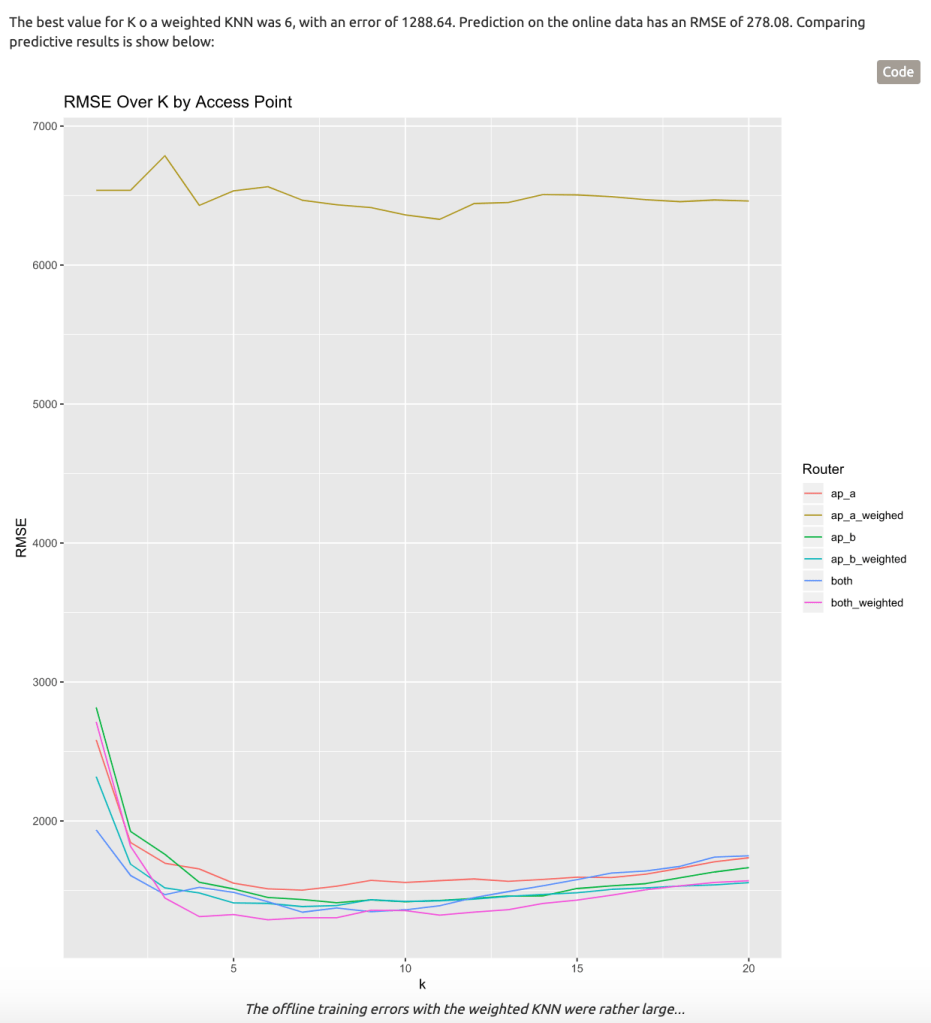
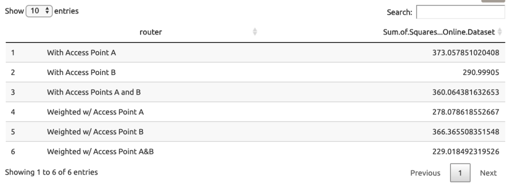
Cross validation for the weighted KNN performs poorly. However, the Weighted model performed the best of all models in terms of prediction, with the lowest error when compared to actuals. Once we dove deeper into the weighted models, it seems that the Weighted Model with Access Points A&B had the lowest among all model with regards Sum of Squared Error which was our key evaluation criteria. This brought us to a sum of square error point of 229 on our prediction testing set.

7 Conclusion

Overall, we were tasked with evaluating which combination of Mac Addresses helped us better predict the location of handheld devices in a building using signal strength and angles. After running six total models to predict the location of Mac Addresses based on the respective signal strength, we found that combining both the Access Point A & B garnered the most predictive signal when we are weighting the signal strength to its distance to the test device. We were able to come to this conclusion by employing cross-validation as well as predicting against the location of the online dataset, and the A&B Weighted model gave us the lowest Sum of Squared Errors. This would make sense as we would have a negative relationship between distance and signal strength and this would help us account for the layout of the building. All of this helps us use signal strength and angles to locate handheld devices within a building.

8 Deployment

With being able to predict the location of users in a building using a wifi connection and access points, we are now able to better understand the usage of our cellular and wifi resources within a building space. For example, if we were to find similar results in a library, we will then know that most of the students are on the west side of the library so that we can boost the wifi capabilities on that side using the unused resources on the east side of the building. From a bigger scale, on Football Game Days, a campus can transmit most of the wifi resources towards the stadium side of the campus using the (likely) unused wifi resources on the library side of the campus. This will help ensure a campus can meet the connectivity needs of its student population without spending Unnecessary amounts of money to manage traffic spikes.

The drawback to this method of using real-time to locate an object is accounting for the fact that objects are typically in people’s pockets or backpacks as they move around the room, so we may lose track of the handheld devices in the room if our data is providing snapshots of x’s around the room rather than labeled users. This could limit our insight capability of being able to see into how specific users interact and move around a building for further analysis. We could correct this by potentially pairing an IP address with the device receiving the signal and including that ip address as a separate column in our dataframe.

9 References

Deborah Nolan and Duncan Temple Lang, “Case Studies in Data Science with R”. University of California, Berkeley and University of California, Davis. 2015. http://www.rdatasciencecases.org