The goal of the Higgs Boson Machine Learning Challenge is to explore the potential of advanced machine learning methods to improve the discovery significance of the experiment. Using simulated data with features characterizing events detected by ATLAS, we classified events into “tau tau decay of a Higgs boson” versus “background.”
The first 10.5 MM rows are trained and validated with a 9:1 ratio and the last 500 rows are tested for accuracy, precision, recall and ROC score metrics, not unlike the classification models you will see on this site. However, using tools such as Tensorflow, we can optimize parameters for number of layers, neurons (units), activation function, batch size, kernel initializer, optimizer, learning rate, epsilon, decay rate, and dropout rate to get the greatest classification accuracy.
The goal of this assignment has 3 key components. The first is to research and get the relevant data from a website by using web scraping techniques. The second is to clean, parse and organize the scraped data into a single dataframe. The final step is to perform an exploratory and statistical analysis on the dataset to help answer a question. The dataset and website in question is The Credit Union Cherry Blossom Ten Mile Run and 5K Run-Walk race results for the female runners in the 10-mile races. The website http://www.cherryblossom.org contains race results from 1999 – 2019, however we will be focusing on the results from 1999 to 2013. Using this specific race and time frame, we are focusing on reviewing whether the age distribution changed among the female race contestants over the years. Using a series of EDA, linear regression, change point analysis, and ANOVA(Analysis of Variance) we found that there was some significant movement in age over the span of the years.
Thanks: Samuel Arellano, Dhyan Shah, Chandler Vaughn
Previously, I worked on building a classifier in hopes to classify the liquor type involved in a sale between Iowa wholesaler to the retailer based on the data of the sale, volume, and location. You can see the results of that classifier here.
In hopes to improve the performance of the classifier, a team and I looked to build a clustering algorithm to locate new variables that can be used to improve the classifier. See the results of our findings and the performance of our ‘improved’ classifier below.
Our job was to build a logistical classifier that predicted the liquor type based on data on wholesale to retail purchases in the state of Ohio in 2019.
Introduction – The Iowa Liquor Sales dataset is an API from Google’s Bigquery which contains the wholesale purchases by retail stores in the Iowa area. The dataset includes the spirit purchase details by product, date of purchase, and location the item was purchased from an Iowa Class “E” liquor license holder (retail stores). The time frame of this data starts from January 1, 2012 through December 31, 2019. As part of the study commissioned by the Iowa Department of Commerce, all alcoholic sales within the state were logged into the Department system, and in turn, published as open data by the State of Iowa. The dataset contains detail on the name, product, quantity and location of the individual container or package sale between the wholesaler (vendor) and the retailer.
Abstract— In this paper, we present how to improve database efficiency and reduce costs by using elastic database pools in software-as-a-service (SaaS) applications. Integral to this is a full tutorial on how elastic pools can be implemented at scale for databases with varying usage patterns while maintaining security, isolation, performance, availability and scalability using the tools available in Microsoft Azure. Underlying this is the concept of a data management strategy, which involve both an understanding of each business case, user’s data, and also the impact of each one’s usage load on the others. Examples we explore include specifying a different database for each customer, co-locating all customers within a single or small number of databases, and setting up a database pool with discrete databases contained therein. Using Azure’s SaaS Wingtip Application, we demonstrated an elastic database pool reducing provisioning costs for a ticketing service provider without sacrificing performance. The methods used can scale to any number of tenants which mimic real world requirements, and which conclude that elastic databases can offer cost benefits in sharing resources.
Index Terms— architecture, availability, Azure, cloud computing, cost management, database management system, DBMS, design, elastic database pool, elasticity, GDPR, General Data Protection Regulation, isolation, multitenancy, noisy neighbor, performance, isolation, provisioning, SaaS, scalability, security, service level agreement, (SLA), software-as-a-service, SQL, tenant, tutorial, WingTip
I. INTRODUCTION
The foundation of cloud computing starts with vendors designing and deploying an application once and making available to customers for a fee for use. This is known as a software-as-a-service (SaaS) application. These application solutions can take a wide variety of forms depending on the business and security requirements of the customer and the databases used to house business-specific data. This can involve customers having their own dedicated application and database as well as a shared application and their database (or tenant) sharing provisioning resources, or somewhere in between.Cloud computing has changed the landscape of application architecture in significant ways. Concepts such as machine learning and big data were once only available to those with access to sophisticated hardware. Now, almost anyone with an internet connection can tap into computing power beyond the scope of their machines. Beyond computing power, users can access the same information in real time more efficiently than ever before. The market has grown because of this, with nearly a 1500% growth since 2008 [1].
The models we focus on are public cloud solutions where customers share a program but have their own unique application instance and require that their data remain isolated. These are popular among cloud computing practitioners and is the focus of this paper due to their nimble capabilities to adjust their size and scope depending on the usage patterns of the application. Because customers co-exist in the same application domain, some unique design considerations must be assured. Fundamental rights such as isolation and security are employed to ensure the data does not fall into unauthorized hands. Service level agreement (SLA) rights include scalability, availability and performance ensure at the quality-level agreed upon by the vendor and end user [2]. Fundamental and SLA rights are non-trivial and lay the foundational criteria we use to assess the performance of our model.
To ensure our model meets the fundamental and service level agreement criteria, data practitioners must define a coherent, vendor-wide plan to handle data created, stored and managed by an organization. This is known as the Data Management Strategy (DBMS) [3]. A possible data management solution includes co-locating all customers within a single or small number of databases and having each customer tenant sharing a single database resource pool. This strategy would be known as a multi-tenant application with multi-tenant pool databases. conversely, you can have different combinations of single tenant application and single tenant databases which involve individual databases and application instances for each customer. Many of the design option combinations either do not meet all the requirements of a SaaS system or cost too much – or both.
In order to design and build these database management solutions, we use Microsoft Azure’s cloud tools to access the computing resources needed in order to scale and test the performance, availability, isolation, and security. While Azure is a relatively new product, cloud computing has been around for decades and allows computer networks to connect and share finite resources to drive greater efficiency. Over time, vendors have turned cloud computing into a commodity with a business model that includes managed services, commodity hardware, metered pay-for-use, and on-demand resource provisioning.
While these business model characteristics all play a role, the concept of on-demand provisioning of resources help differentiate Elastic Database Pools from the other solutions. In a database pool, tenants share computing resources (such as bandwidth and CPU) known as provisioning and tenants only pay for what they use. The database pool design option is of great interest because it may provide a way to both meet key fundamental and SLA requirements while costing less overall than if we had separate provisioning settings for each database. Elastic database pools are also ideal for managing databases that have variable performance strain (or load) and have a high likelihood of scaling. Companies such as Cyberesa have used database pools in a similar fashion and saw costs decrease.
In this paper, we explore these issues and provide a tutorial of how to set up and use an elastic database pool in Microsoft Azure using Azure SQL databases. As a demonstration of our strategy in effect, we employed the Wingtip SaaSTicketing application within Azure. As a prerequisite to the tutorial, we provide a detailed walkthrough of how to set up Azure and PowerShell. We then provide a guide of how to get started, establishing the tenants in your pool, loading our elastic database pool with database activity, restoring a lost tenant and accessing the cross-tenant reporting data. Using Elastic Pools, we tested the performance of the database at load scenarios at a scale that mimics real world conditions.
I. Software-as-a-Service (SaaS) Applications
The SaaS application model has grown in popularity [4] over the last several years. Using this model, vendors can deploy a software application once to make it available to customers. Customers license the software by paying a periodic fee, typically monthly and/or by number of users, in order to access the software. Examples of popular SaaS applications include: Adobe Creative Cloud, Microsoft Office 365, GitHub, and even the statistical software SAS On Demand. These clouds can be public or private, depending on the business goals [5]. Public clouds are more popular and are ideal for applications with a high degree of elasticity and range of scalability needing a greater reach. Private clouds are more ideal for workloads with intense security and resource needs while being able to support a shared infrastructure. For this paper, we focus on public clouds as they are more popular and are better suited for varying elasticity.
Cloud technology is particularly useful for deploying a SaaS application because of its elasticity, multitenancy, and scalability. These features have grown to allow SaaS to be the standard bearer for modern enterprise computing and collaboration, and these can take many shapes with regard to how customers can have their own or shared database, tenant, and application to meet their business objectives.
A. Database
One of the key features of SaaS applications is the access of users to databases owned and managed by the vendors they are using. For the purposes of this paper, we define databases as a structured set of data that is stored within a CPU and is accessible in various ways. In practice, customers can share a database with another customer or have their own [6].
Each database used in a SaaS model is known as a tenant [7] in much the same way that each resident of an apartment complex can be considered a tenant. In practice, tenants can share a database with another customer or have their own. A multi-tenant database strategy involves companies employing a third-party provider to house their data in a shared database management service (as opposed to a more traditional model wherein users install software independently from each other on their own computing and networking equipment).
B. Application
The nature of a SaaS model starts with the concept of an application where a program is designed to address a customer’s service requirement. These applications can be built for a single customer per instance, built for a single instance to be shared by many customers, or built so that each customer shares an application, but is served a unique instance to them. While single tenant applications are still practical for large clients, one of the key flaws in the single tenant method was the overall low utilization averages for each database. One case showed that the CPU utilization can be as low as 4% across 200 database servers. Modern multi-tenant database models correct those utilization needs with their shared resource structure [8]. These single-, multi-, and pooled-tenant databases can be paired with different combinations of single and multi-tenant applications. We focused on those needs and structure here.
II. SaaS Data Management Features
The database multitenancy nature of SaaS applications carries with it important offerings that must be factored into any SaaS application design. These offerings are necessary in order to ensure fundamental rights such as isolation and security as well as service level agreement (SLA) offerings like scalability, availability, and performance. Database management system practitioners need to be dynamic in how they provision resources so that they can meet their job needs without violating SLA offerings for a project to maximize revenue [5]. Because customers have limited control over the infrastructure, database, and application deployment, the SaaS vendor must provide these service offerings to its customers.
A. Security
Each customer of the SaaS application needs security. Security in this context includes protection from software exploits and common attacks. A security breach can carry significant commercial consequences. For example, in 2015, the makers of MacKeeper “acknowledged a breach that exposed the usernames, passwords, and other information of more than 13 million customers” [9]. Customers might be exposed in ways that carry financial, reputational, and opportunity costs. Customers are connected by virtue of their all being part of the same application. As a result, if one customer is compromised, it is likely that all the others could be, too. Because a breach could easily impact many or all the customers who are subscribed to the SaaS service, market and regulatory consequences for the SaaS provider could be severe. Due to these factors, security is of paramount importance and must be considered carefully in the SaaS application’s design.
B. Isolation
Isolation carries increasing importance for everyone and is necessary to safeguard privacy. Security breaches can compromise isolation, of course, but there are additional risks in a SaaS service. Since all customers are logically part of the same application, there might be risk of data leakage, wherein one customer’s information might inadvertently be made visible to another customer. Beyond the obvious market implications of a product that offers poor isolation protection, new regulations such as the General Data Protection Regulation (GDPR) [10] provide significant penalties for vendors to uphold database isolation. The importance of privacy therefore leads us to a key requirement of any SaaS system – that of customer complete isolation between customers.
C. Scalability
Customers using the SaaS application have different needs as time goes on. Commonly, seasonal spikes occur. For instance, consider a SaaS service that provides web sites that other companies, in turn, expose to their own customers for ecommerce purposes. Various industries tend to have differing load peaks, a phenomenon known as seasonality. For example, a retailer could experience spikes in volume around the Christmastime holidays. A flower shop might have spikes around Valentine’s Day and Mother’s Day. A lawn and garden supplier might see its highest business in the summer, and so on. The SaaS application needs to be able to dynamically scale in order to meet the demand of these usage spikes without affecting other tenants.
The addition of new customers in and of itself could cause scalability issues. The system must be able to dynamically provision additional resources as needed to meet the demand of new customers. Inversely, if customer load or demand falls, the system should deallocate resources in order to save on cost.
D. Performance
Performance needs to be consistent in accordance with the SaaS provider’s SLA. For instance, a seasonal spike at one customer should not only be met with enough performance to guarantee that customer’s requirements, but such a spike should also not affect any adjacent customers in the tenant. This is known as the “noisy neighbor” problem. It is the job of the SaaS application to manage this performance transparently to its users.
E. Availability
Availability is a service level agreement condition where a specific resource or value is available and accessible by the customer. Availability is measured in terms of a time percentage of the accessibility of the database, and it can also sometimes be measured in hours. Customers should be able to easily access the database while logged onto the database, so, in cloud computing, availability is paramount. Availability with fault tolerance in both accurate analytical querying and in transactional systems with Atomicity, Consistency, Isolation, and Durability (ACID) properties being ensured [11].
I. Potential SaaS Database Management Solutions
Meeting the offering requirements for a robust SaaS application involves careful design. A few options are available through varying combinations of single or multiple application and database tenancy, as discussed previously. These options, however, provide different services for the system. Others may meet requirements but at excessive cost. We weigh the various options in this section and determine a design strategy.
A. Multi-Tenant Application with Multi-Tenant Database
In this approach, a single application hosts all users of the system (i.e. a “multi-tenant” application), and a single database is used for all user data (i.e. a “multi-tenant” database). A key benefit of this approach is its low cost. If only one application instance and one database is required for everyone, then the SaaS vendor needs to only pay for those single resources.
However, this approach does not meet all the requirements. In fact, it risks not meeting any of the requirements. First, there is no isolation since all customers are saved in a single database. The risk of information leakage is high. In addition, there are risks to security (a breach could expose all customers in the single database) and performance (noisy neighbors could affect other customers). As a result, this is a poor design choice for a SaaS application.
B. Multi-Tenant Application with Single-Tenant Database
This strategy takes the previous design and provides a separate database for each tenant. Such a decision certainly provides isolation since each tenant is in its own database, and it also enhances security, since any data breach would affect only the customer who was breached. However, it is not perfect, and some data leaks can be caused through malicious tenants and virtual machine instances [12].
However, this solution would be very expensive. Database resources tend to be expensive, and if you need a separate database for each tenant, the cost grows very quickly. In addition to cost, scalability suffers because scaling might potentially need to occur at more than one – or all – of the databases at once. Such management overhead would be unwieldy. Imagine that a particular SaaS application has millions of users. You would need millions of databases in this scheme!
C. Single-Tenant Application with Multi-Tenant Database
If we flip the approach around and provide each customer with its own application but sharing a database, app isolation would help with security, and going back to a single (or few) databases reigns in cost. Scalability is also improved because we are only using a single database.
However, we are back to the original key problem with having a single database – no isolation. A coding error or security breach could easily expose one user’s data to others.
D. Single-Tenant Application with Single-Tenant Database
In this design, each customer gets its own application and database. Not only are all requirements met, but this solution provides maximum isolation for security and isolation. Unfortunately, scalability is challenging, as in other single tenant solutions. Worst of all, the cost would be greater in this model than in any of the other models!
E. Single-Tenant Application with Pooled Single-Tenant Database (EDP)
Now let’s examine using the previous solution with one modification: instead of using a separate actual database per user, we use a separate logical database per user. Those logical databases are grouped into one or more elastic database pools. These pools are groupings of databases that allow loads across all the databases to be averaged out.
Because the databases are still separated, all of the requirements we have discussed are met in this scenario. However, because they are billed and managed as a block, cost is far lower, and management is far easier.
II. Microsoft Azure Cloud Services
The origins of cloud computing date back to the 1960s. One of the first cases of a shared resource network comes from an IBM computer scientist, Bob Bemer, who designed a program that re-provisioned time that was not being used while other computer scientists and processors were waiting for an I/O and allocated it to users who needed it more urgently. This allowed multiple people to use the systems at the same time while also driving efficiency in lowering the average time needed per user. This time-sharing software eventually led to mainframe, transaction, and grid computing systems as the key resource categories for programmers to share. Azure is the overarching brand name for the cloud-computing service offered by Microsoft, which is one of the market leaders for this type of service along with Amazon’s AWS and Google’s GCC. Azure is an ever-expanding toolbox of various cloud computing services. Azure gives the freedom to build, manage, and deploy applications on a massive, global network using a selection tools and frameworks.
Cloud-native computing with Azure is defined with several key characteristics, such as enablement of a variety of managed platform services (such as virtual machines and data storage), constrained multitenant services running on commodity hardware, on-demand provisioning of resources, and metered pay-for-use in a short term rental model, which is enabled by horizontal cloud scaling [13].
With these characteristics comes many well-documented advantages, including cost management, elasticity, scalability, and multitenancy. Azure offers a solid implementation toolkit of an elastic database pool service that even allows users to scale their demonstration database to real world sizes. Utilizing the cloud service allows us to focus on the potential benefits of elastic pools rather than creating, installing, or managing the underlying technology. Such benefits in this context realize many of the key benefits of the cloud in general, especially that of multitenancy, elasticity, and scalability [14].
Among the key benefits of cloud computing, scalability is one of key difference makers to an advanced outsourcing solution. As computing power has grown more advanced over years, more computers are able to access sophisticated applications via virtual machines. The ability to link via a shared network and database is integral to the modern computing landscape. To achieve scalability in your database management strategy, the costs to ensure performance, availability, and scalability of each database are a real concern, and elastic databases are a practical solution to manage resource provisioning while also being easy to implement [15].
III. Elastic Database Pools (EDP)
As of November 2019, relational database management systems make up 75% of the popularity of all database types. EDP works with relational database managements systems [16], thus, pooling technology is extremely applicable given the current landscape of the database market. The basic idea behind an EDP is that one database pool “holds” many discrete logical databases. Each database is assigned to a single user or customer in order to meet SaaS requirements. Performance and provisioning occur at the pool level. The key observation that of which this product takes advantage is that not all users need all their database performance capabilities at the same time.
A. Variability
Following up on our earlier ecommerce example, consider the retailer who needs more resources at the end of the year and the flower shop who needs them in the spring. Because one user’s peak is the other’s normal or down time, capacity is available for both when they need it.
The same idea holds true for usage patterns in other time scales. For instance, perhaps one customer needs access during business hours so that their employees can do their jobs. Another customer might need more resources at night for batch processing. Because one user’s peak usage complements the others, we can pay for the average case of the resource from our cloud provider rather than the maximum (i.e. worst) case, which is precisely what was needed in the other models. Cost goes down as a result.
B. Scalability
The underlying nature of the cloud supports scalability, and a cloud based EDP takes advantage of this feature to provide scalability when needed. For instance, consider if some non-trivial subset of users all needs their maximum-usage performance at the same time. Maybe a large percentage of customers are retailers, and its holiday time. The pool can be configured to dynamically scale as needed in this scenario.
This may seem counter-intuitive to the basic premise of averaging usage needs across customers; however, it would be naive to think that the system would never need to exceed its average case, so we should plan for such a contingency. Because we can scale beyond the average case when needed and return to the average case when the need has passed, we can meet SaaS SLAs and still save on cost because we only provision the extra resources when they are actually being used rather than all the time.
C. Identifying Candidates for Pooling
It’s important to consider usage patterns when designing the system. For instance, if it is likely that all customers might have similar peaks and valleys in their needs, then pooling might not provide as much cost savings. A better approach might be the single database model with automatic scaling, though, of course, the cost would be higher.
The best scenario is one where users roughly balance out each other’s needs. One user’s needs are high while another’s is low and vice versa. It may be possible, especially with a large SaaS implementation, to place complementary usage patterns on the same server. Additionally, provisioned servers can replicate that pattern with other complementary users, and so on.
Even if usage can’t be predicted up front, a well-written application can monitor usage patterns and migrate users (in their off-peak times) automatically to other servers to gain the benefits of average-case usage. This sort of automatic balancing should be a component of a robust SaaS application. The general rule of thumb is that spikes of at least 1.5 times the average are good candidates for an EDP.
D. Proactive SaaS Resource Allocation
Once the initial SaaS application is designed, the next step should be to add algorithms that can proactively allocate future resources based on historical demand, accounting for the fact that each tenant has its own demand patterns.
Historically, database administrators used prediction models in attempt to forecast the need for database provisioning on a proactive basis. This involved machine learning techniques to extrapolate future data using historical performance data. Over time, this has been adapted to use in conjunction with reactive elastic database pools to identify which variables are key predictors of peak or depression performance [17].
Among previous works that discuss elasticity in multi-tenant databases, in a study on predictive replication [18], authors introduce and propose an approach that uses forecasting methods to provision future workloads on cloud database systems. With this prediction, they are able to algorithmically allocate or disseminate resources accordingly to reduce costs and maintain performance SLA requirements.
After using prediction models to characterize the workload of a cloud database system, they were able to compare those results to a more reactive approach. Between the two approaches on a multi-tenant database, the forecasting approach reduced the number of SLA violations by way of elastic replication of database resources. With these results, a key limitation was that the change in resource needs can make prediction difficult to pin down reliably.
Incorporating these techniques into a SaaS application takes advantage of the elasticity of cloud computing and predictive power of machine learning models to make sure resources are available when they are most needed and deallocated when they are not to save on cost.
IV. Actual EDP SaaS Implementation Example
To get a sense of the benefits of EDPs in the real world, let’s consider Cyberesa [19], a Tunisian software vendor for the hospitality industry. This company processes over 10,000 bookings a day, and any downtime could result in a lost sale. At scale, that could mean a loss of $240k on a high season. Cyberesa used Azure Elastic Databases to help provision the load of the database activity between daytime and nighttime. This allowed them to auto scale settings based on CPU performance, use automatic backups, and use staging slots for an easy, streamlined deployment cycle. The use of Azure improved performance and allowed Cyberesa to reduce each single database requirement from 50 DTUs to 20.
V. EDP Tutorial
It is useful to see this technology in action, so the tutorial includes a written walk-though, a short live demo, and a more in-depth recorded demo, which is available here: https://youtu.be/3XYWxCjOefI.
To demonstrate EDP, we utilized a sample Azure application written by the vendor (i.e. Microsoft) for this purpose. This application is called Wingtip SaaS. The repository can be found here: https://github.com/Microsoft/WingtipTicketsSaaS-DbPerTenant. This which allows the interested reader to reproduce or expand upon the demonstrations of this tutorial. Wingtip simulates a ticket-processing service and demonstrates EDP for several types of ticket-processing vendors.
The demonstration covers creation, provisioning, schema management, monitoring, and support activities. In addition, we demonstrate how EDPs can be used to add users and scale resources. The tutorial conveys the benefits of using this technology, design considerations (nothing is free, after all), and possible downsides as well as a good sense of how to get started and next steps to implement EDP in other SaaS applications.
A. Prerequisite – Azure
Since we are using Azure for the tutorials, it is necessary to have a basic understanding of the technology. This tutorial assumes no prior knowledge of Azure or cloud services. It begins by showing how to log in to the Azure portal and how to obtain some free Azure credit in order to follow along with the demonstrations.
The scope is limited to those services that are used as part of the tutorials. This includes the demonstration web application (which uses App Services, App Service Plan, and Traffic Manager), Azure Resource Manager (ARM) templates, and the demo databases (which use Azure SQL Database and SQL Elastic Pools). It also includes certain limited features of those services, such as provisioning, monitoring, and configuration.
B. Prerequisite – PowerShell
The tutorials rely on PowerShell scripts to accurately execute the demo steps, and many of those steps involve repetitive and/or time-consuming activities, such as provisioning dozens of databases. Because of this, it is necessary to have a basic understanding of PowerShell to follow along. No prior experience in PowerShell is assumed; however, it is helpful to have some basic experience in any programming language or environment in order to understand the basic concepts.
The tutorial begins with how to launch and work with the PowerShell environment. Then, it describes some basic commands and their syntactical structures. Next, scripting staples like variables and control structures are demonstrated. Finally, basic data structures used in the demo scripts like arrays and hashes are shown.
C. Getting Started
This tutorial shows how to get the Wingtip Ticket Processing SaaS demo application set up and usable for all the tutorials to come. It covers provisioning the complete Azure environment for the Wingtip application using PowerShell. Once provisioned, a brief tour of the newly-created artifacts provides hands-on illustration of the starting state of the application, which initially consists of three tenants. Then, a load is placed on the application, and a new tenant is provisioned while the load is applied to demonstrate that the system can stay “up” while tenants are created.
D. Tenant Provisioning
For the tutorials to come, there needs to be at least 20 or so tenants running in the application. This tutorial takes advantage of this need by including how to automate the provisioning of new tenants in PowerShell. It also goes into greater depth on exactly how each tenant is being provisioned in PowerShell. Once all of the new tenants are provisioned, a moderate, steady load is placed on all of them, and we explain how the load is generated using SQL and PowerShell.
E. Pool Load Management
This tutorial ultimately demonstrates how to scale elastic pools up and out. It also shows how to scale individual databases in the pool. However, in order to see how variations in load affect the performance of the pool, it is first necessary to understand what monitoring tools are available. Therefore, this tutorial begins by showing how to monitor the pool as a whole and individual databases within that pool. The monitors use the Database Transaction Unit (DTU), an amalgamation of multiple performance measures including CPU and disk times.
Next, the tutorial demonstrates how to set up alerts and goes through a few of the metrics available for alerting as well as various thresholds and communication options. With the sample alert in place, load is increased to about double its previous level along with long spikes. The result of this load is shown on the pool and databases, and the alert is shown to have been triggered.
With the pool at its maximum performance capability, the tutorial demonstrates scaling up by showing how to double the DTU capacity of the pool and the effect this has on better handling the heavier load. Then, the tutorial adds a second pool and moves about half of the databases into it to show scaling out. Finally, a very heavy load is placed on a single database, and the tutorial shows how to scale up just that one database without affecting the rest of the pool.
F. Tenant Recovery
This tutorial demonstrates how to recover a tenant without bringing any other tenants down or affecting any other parts of the application. First, some events in the application are shown, and then those events deleted and verified as being gone. Then, the backup database that Azure automatically keeps is restored for that tenant only. All other tenants are running with load at the same time. Finally, the missing event is shown to have been restored.
G. Cross Tenant Reporting
This tutorial shows how to report across tenants for application-wide insight. To do this, hundreds of tickets are first automatically purchased for each of the tenants in the system. We then validate that the tickets were successfully purchased and that the information is available in a special database in the catalog database server. This database has information from all the tenants (each of which have their own independent databases), which allows the information to be queried collectively. Finally, queries are executed against the catalog reporting database, and the resulting execution plans are examined to see how the database executes queries across tenants.
Leon Erlanger. (2005, May). Software as a service a field guide. Network World Canada.Volume 15 (Issue 9), 16-17.
Mary Johnson Turner. “Multicloud Architectures Empower Agile Business Strategies”, Nutanix. August 2016.
Van Arkel John H et al. “DATABASE.” 7 Jan. 2016: n. pag. Print.
Houda Kriouile, Bouchra El Asri. (2018, July). A Rich-Variant Architecture for a User-Aware multi-tenant SaaS approach. International Journal of Computer Science. Issues. Volume 15 (Issue 4), 46-53.
Monica C Meinert. (2018, May). GDPR. American Bankers Association. ABA Banking Journal. Volume 110 (Issue 3), 30-33.
Curino, E. P. C. Jones, S. Madden, H. Balakrishnan, “Workload-aware database monitoring and consolidation”, Proc. SIGMOD, pp. 313-324, 2011.
Brian Krebs. (2015, December). 13 Million MacKeeper Users Exposed. Krebs on Security.
Shamsi, Jawwad et al. (2013) Data-Intensive Cloud Computing: Requirements, Expectations, Challenges, and Solutions. Journal of Grid Computing. [Online] 11 (2), 281–310.
Mundada, Yogesh, Anirudh Ramachandran, and Nick Feamster. “Silverline: Data and Network Isolation for Cloud Services.” 2011.
Bill Wilder. “Cloud Architecture Patterns: Using Microsoft Azure,” O’Reilly. 2012, 9-10.
Danai Gantzia & Maria Eleni Sklatinioti. “Benefits of Cloud Computing in the 3PL industry,” M.B.A Thesis, Jönköping International Business School, Jönköping, 2014.
Luis M. Vaguero, Luis Rodero-Merino, Rajkumer Buyya, “ACM SIGCOMM Computer Communication Review”, Hewlett Packard Labs, Bristol, United Kingdom, Volume 41 Issue 1, January 2011, Pages 45-52.
Gustavo A. C. Santos, Jos´e G. R. Maia, Leonardo O. Moreira, Fl´avio R. C. Sousa, Javam C. Machado. “Scale-Space Filtering for Workload Analysis and Forecast,” IEEE Sixth International Conference on Cloud Computing, Fortaleza, Brazil. 2013.
Flávio R. C. Sousa, Leonardo O. Moreira, José S. Costa Filho, Javam C. Machado. (2018, February). Predictive elastic replication for multi‐tenant databases in the cloud. Concurrency and Computation Practice and Experience. Volume 30 (Issue 16)
This Repository is for Clark Consulting’s Attrition and Salary analysis for Frito Lay Employees
Introduction The modern workforce in the United States is becoming more fluid than ever before. As the cost of living in the country continues to increase, wages are remaining stagnant, as reported in the latest economic trends. A result of this, we are seeing more employees shift between companies after just a few years and using the larger pay raise associated with switching jobs (as compared to staying put a single job) as a way to bolster their income to make a living.
To combat this trend and potentially get a closer feel of the status of each employee and their potential for attribution, we are going to conduct a data analysis to identify trends in the employee base job titles, overall sentiment as well as salary with hopes to be able to predict which employee is likely to leave the company and what salaries are associated with the employee’s current standing.
Repository Contents: CaseStudy2-data.csv – Traning dataset of Frito Lay Employees (includes salary and attrition) CaseStudy2CompSet No Salary.csv – Includes Testing Set of Frito Lay Employees (does not include salary data for prediction) CaseStudy2CompSet No Attrition.csv – Includes testing Set of Frito Lay Employees (does not include Attriton) Codebook.html – HTML version of description of data for Training and testing sets DanielClark_DDS_CaseStudy2.Rmd – R Markdown file of data cleaning and analysis DanielClark_DDS_CaseStudy2.html – HTML knit of data cleaning and analysis process MSDS_DDS_CaseStudy2.ppt – PowerPoint used in presentation to FritoLay executive team
U.S. Beer Market is growing more saturated with small-scale breweries taking more market share and shelf space from the National Domestic Beer Manufacturers. Newer brands are covering the spectrum of bitterness and gravity size, and they are beginning to spread across the country. As AB Inbev is looking to test the waters in the craft brew space, understanding the local trends with these factors may help open market deficiencies as well as locations that may enjoy a bitter beer over others. This information can help guide AB Inbev with insight to opening new chains of micro-brews around the country.
Repository Contents:
Brews.csv – Unique beers from microbrews names, ABV, IBU &
Breweries.csv – Location and ID data on microbreweries
Codebook.rmd – Description of data for Brews.csv & Breweries.csv
Codebook.html – HTML version of description of data for Brews.csv & Breweries.csv
CaseStudy_01_Grace_Daniel_Final.Rmd – R Markdown file of data cleaning and analysis
CaseStudy_01_Grace_Daniel_Final.html – HTML knit of data cleaning and analysis process
.ppt – PowerPoint used in presentation to Anheauser-Busch executive team
With the NFL pushing nearly $8.2 billion in revenue in 2017, the league is becoming bigger business than ever before. With more at stake for teams to be successful, there is a massive emphasis placed in scouting college athletes and finding those with the greatest aptitude towards performance in a professional football setting.
This is not an exact science by any measure. For all the many success stories of diamonds being selected in the rough to go on to have great careers in the NFL, there have been some famous missteps by teams investing their future into a new player who ultimately did not pan out. Fans of the NFL have a not so delicate way of referring to these players as “busts.”
The flagship event in the scouting process in professional football is what is called the NFL Combine. This 3 day long event typically held in Indianapolis, IN, is a gathering of all the top athletes in college football to demonstrate their strength, speed, agility while also getting their official heights and weight data for teams to analyze when making their selections for the next year.
One of the most popular events at the combine is a 40 yard dash, known as the “Forty”. The reason why it is most popular at these events is not only because it’s exciting to see these athletes running 25 mph across a football field, but it also is considered to be one of the most reliable measures of future performance in the scouting process. The logic makes sense, as you can teach technique and strength all you want within a player, but if they can’t get from A to B faster than the other guy, then they are not going to be able to make a play.
For this project, we are going to review about 17 years of combine data (dating back to the year 2000 when electronic timing for the Forty was implemented, and see if we can detect patterns within player attributes to figure out what would generate the fastest 40 time among prospects.
Data Description and Overview
Data Overview
The dataset includes a population of over 6,000 NFL draft prospects that appeared and tested in the combine from 2000 to 2017 with 15 explanatory variables describing some detail about the players, including position, height and weight as well as some of the combine performance data including how many reps they could bench press 225 pounds, vertical jump, broad jump and the shuttle drill. The data came from Kaggle and includes the 40 times for the players which range from 4.24 (the fastest time ever recorded) to 6.05 (the slowest time ever recorded). The goal of the assignment is to see if we can take some of the other explanatory variables to predict the forty time of each player. Including the 40 time, below is an explanation of some of the other variables involved in the study.
Combine results reported in this study Include
40-yard dash
The 40-yard dash is a test of speed and explosion. Starting from a three-point stance, the player runs 40 yards as fast as possible. Times are recorded in 10-, 20-, and 40-yard increments.
Bench press
The player’s goal in this exercise is to bench press 225 lb as many times as possible. With the exception of quarterbacks and wide receivers, all players participate in this test of upper body strength.
Vertical jump
To measure the vertical jump, a player stands flat-footed in front of a pole with a number of plastic flags sticking out. The player then jumps from a standing position and swats as many flags as he can, thus enabling the judge to determine how high the player can jump. This exercise is considered important for wide receivers and defensive backs, where jumping ability is a critical skill.
Broad jump
The broad jump measures how far a player can jump from a standing position. This drill is most important to positions that use lower-body strength (such as offensive and defensive linemen) to gain an advantage.
Cone drill
In this exercise, three cones are set up in a triangle shape with each cone 5 yards apart. Starting in a three-point stance, the player sprints in a predetermined route among the cones. This exercise tests speed, agility, and cutting ability.
Shuttle
In this exercise, the player starts in a three-point stance and runs 5 yards in one direction, 10 yards in the opposite direction, and then sprints back to the starting point This exercise tests lateral speed and coordination.
Population of Interest
The population of interest in our study are the 6000 participants in the NFL combine. These participants are former college athletes from the United States with a great skew towards athletes who played varsity football in college. Per the NFL rules, the athletes need to be at least 3 years out of high school, so the majority of the data is from athletes who are ages 20 and over.
There is also an invitation process for college athletes, so the best of the best players in the NCAA are only invited to the combine. Out of over 10,000 players active in the NCAA, only 335 are invited to the combine each year.
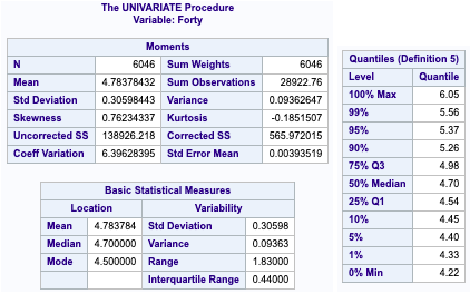
EDA
Looking at our key response variable in our data set, the forty time, we can see that there is a small variance between 40 times with 75% of the data being below 5 seconds (which is much faster than you or I could run). We can see the mean 40 time is 4.78 with a median of 4.70, which would suggest there is a right skewness to our data.
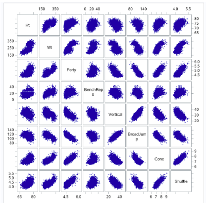
Fig 0-1 (workout scatter plots)
Looking at the combine performance data, we can see some clear positive/negative relationships happening between players who perform well in some events and their performance on others. For example, we can see that players who have a lower 40 times tend to not be able to bench press as many times, and we can see that faster players do not seem to jump as high or as long. Which may be related to height, it appears that shorter players are faster, per the scatter.
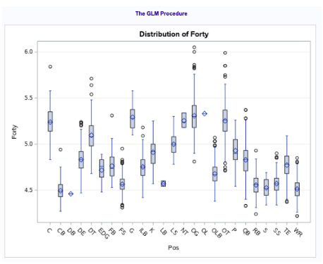
In Fig 0-2, we can see the 40 time by position group. Here, we can see that the faster positions in the NFL are DB, WR, S and CB, while the slower positions are offensive linemen (who are known for being bigger players) such as Centers, Guards and Tackles.
Fig 0-2: Analysis of Variance between positions
Looking at an analysis of variance between position and 40 time (fig 0-3), we can see the distinction between positional roles on a team and how fast the players can run. Offensive linemen positions (OG, OT, G, C) as well as the defensive nose tackle position all tend to have slower 40 times with means of 5.25. While slower, this makes sense because these types of positions tend to favor power over the other positions, which focus on speed and separation. The faster positions we tend to see are Cornerbacks (CBs), Safety’s (S), Running Backs (RBs) and Wide Receivers (WRs) with a mean forty time of just over 4.5.
Analysis
Restatement of Problem
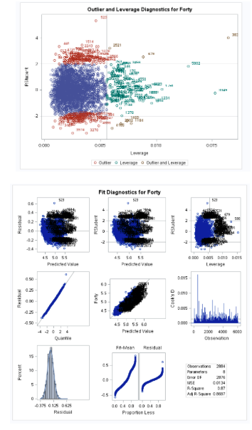
The primary purpose of this study is to examine some of the measures that are part of the NFL combine each year and see how they can go to predict the 40 yard dash time, which is considered to be the flagship measure of a player’s capability in the NFL. This will notably include the performance measures of non running events as well as positional attributes within the players. As we see in fig 0-1, 40-yard dash ( forty) has a linear positive relationship with weight, height, bench press, cone drill, and shuttle. In addition, it has a strong negative linear correlation with Vertical jump and Broad jump. As we see in fig 1-0 and 1-1, there are some outliers or leverage or both, but one observation has high in magnitude.
In figure 1-0, we can see observation 3878 is a high leverage point with regards to 40 time. Doing some research, we can see this observation is of Isaiah Thompson, who is known for having the slowest 40 time in the history of the combine at 6.04 seconds. Using an NFL analyst, Rich Eisen forty time of 5.97 as a control time (since he was 48 years old and wearing a suit), we can use this as cause for dropping Isaiah Thompson’s time due to his performance being not up to the standard of performance that a player would need to be at to be someone who was invited to the combine.
After dropping Isaiah’s time, we can see that our regression model better meets the assumptions that we would need to satisfy our regression model, even without transformation needed to our dataset.
Normality – reviewing the histogram plot available to us, we can see that while there is a slight right skew. However, it doesn’t seem significant enough to warrant us applying a transformation to our data. This right skew is natural since it is much easier to get a slower 40 time than it is to get a sub 4.3 forty.
Constant Variance – regards to constant variance, we can see through our residual analysis that we have a pretty consistent cloud at the low values and a little more scattered at a higher value. However, after trying a transformation of a log of the 40 time, we cannot see a significant improvement.
Linear Trend – The linear trend analysis shows all the data fits pretty cleanly on a single regression line.
Independence – While the fact that many of the players in the combine have the same coaches, which may have a covariate effect on scores, it doesn’t seem significant effect to be troublesome in our analysis. So we will assume independence moving forward.
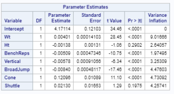
Looking at the Variance inflation factor in Figure 1-1, we are not seeing any evidence of collinearity between the factors we will use for our study. Typically, we would be concerned if we see any VIF scores at above 10 for a variable.
Model Performance Metrics
All explanatory variables are initially coded into the model, the model worked under the assumption that NA’s were relevant data and the model would weed out irrelevant NA’s not reflective of missing data, which is an assumption that would carry over across all our models.
After going through the model assumption and model assessment we come to the model selection. Using the dataset, we would like to explore the factors that contribute to a good performance in the response variable ( Forty). We will attempt to create a predictive model to accurately predict the response variable Forty using multiple selection methods, including stepwise selection, LASSO and LAR model.
In the variable selection process and fit diagnostics we haven’t done any variable transformation as conformity to linear regression model is achieved through multiple benchmarks stated in the previous sub chapters.
To filter the best candidate regressing variables we used GLMSELECT procedure cross validation was used as our selection criteria, with no stop criteria. Cross validation is a more effective significance measure because of how it “leaves out” observations as they are examined, to validate the significance of variables at each validation.
Below is a table outlining some of the performance measures of the model selection methods that we used
Predictive Models Adjusted R Square CV PRESS
Stepwise .86 38.65
LASSO .86 38.66
LARS .86 38.66
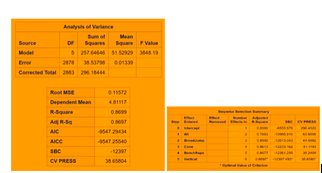
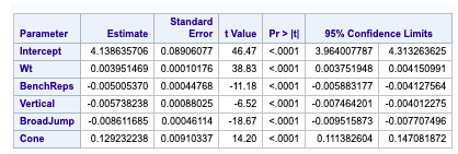
Fig 2-1: Stepwise Regression Technique with CV stop (leaves shuttle out of our final model)
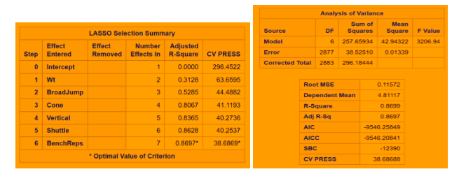
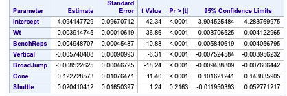
Fig 2-2: LASSO regression technique with CV stop
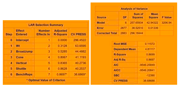
Fig 2-3: LAR regression technique with CV Stop
Fig 2-4: Confidence limits for LAR and LASSO
Fig 2-5 Confidence Limits for Shuttle
The minimum CV press value for the forward selection is given Dependent mean is the mean of the response variable. The Adjusted R Square (Coefficient of determination) and R square values are the degree of measurement of how the response variability is explained to the predicting variables ranging from 0 to 1 where the closer to one the better for adjusted R. The mean Squared Error ( MSE) : For prediction is simply the average of the squared deviations between the Fitted values and the observed data. In our model selection run down the three model selection show pretty much similar RMSE. I used CV press as a model KPI because Cross validation though It is error criterion not selection criteria but it’s helpful when paired with Selection criterion breaking the data into training data set and test data set to get a more accurate assessment of the predictive accuracy of a model. Other selection criterion AIC ( Akaike’s information criterion) which denotes how well the model ( log likelihood) plus how complex the model ( penalizes the model fit by the number of regressors is also displayed for all the three section techniques. BIC ( Bayesian Information criterion) also called SBC is part of the descriptive statistics. For our comparison we choose adjusted R square paired with cv press as a good indicator to pick the best selection model as shown above in the table. Looking at the confidence limits for LAR and LASSO model as well as the Stepwise model, we can see that the addition of the Shuttle Drill would make a marginal change to the linear regression line.
The final Model (custom model)
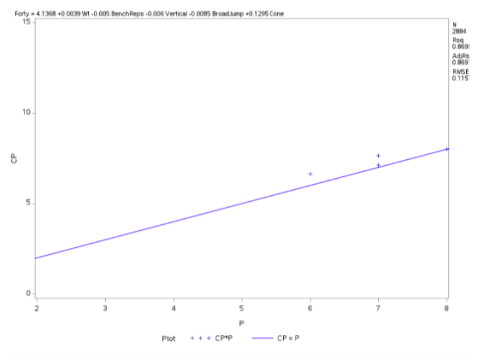
The best candidate predictors that dictate how well the response variable is regressed by the candidate or indicative variable is fitted below with corresponding coefficients in linear fashion.
How the 40-yard dash ( test of player speed and explosion ) is regressed by the prediction variables like weight of the player , Bench press( count of bench pressing 225lb) , height of vertical jump , Broad Jump( how far player jump from standing pose) , cone drill ( as a measure of player agility )
Fig 2-4 Regression Procedure
Conclusion
After tweaking the dataset to remove an outlier time for forty (which we justified due to the player performance not being considered up to standard with the athletes that are typically invited), we have been able to successfully build a regression model that can predict Forty time performance based on the performance of other events at the combine.
After implementing thress regression modeling techniques (Stepwise, LAR, LASSO), we were able to garner successful model fitting with an adjusted R^2 value of 0.8697 and a Root Mean Square Error of 0.115, which is strong enough to show success of the predictive ability without being overfit to new data. This was support using cross validation stopping techniques when running the model selection procedure.
With all that said, we would consider selecting the Stepwise selection procedure as the strongest model because it is able to achieve the same R^2 and RMSE value while using less variables and it’s AIC value is slightly lower.
For further study beyond the scope of this course, we would love the opportunity to access some of the data from the player’s performance from college to predict a player’s 40 time, and potentially use that information to predict future player 40 times based on their college performance data. If this becomes reliable, the NFL can save millions of dollars in resources to assess player performance across the college landscape without the costs to hold events to have players run the 40.