Introduction

As housing plays a major role in the stability of the United States economy, being able to get a handle on the market demands as it relates to housing quality and the price will help business and local governments predict change over time. As one of the largest recessions in American history occurred due to major fluctuations in the housing markets, being able to use data science tools to predict sale prices of homes will be extremely useful in managing resources and understanding major market predictors among home buyers and sellers. Daniel Clark and Robert Hazell will be using the 2006 – 2010 Ames housing data to explore the relationships of the home sale price with other factors, and hopefully predict with accuracy how much a house will sell for when using the data to our advantage.

Data Description and Overview

Data Overview

The data set includes a population of 2930 homes that were sold in Ames, Iowa from 2006 – 2010 with 80 explanatory variables describing each (all of which includes information such as sales price, lot size, pool area, condition, overall quality, etc) which would go into assess home values within that market. The data is available on Kaggle in two sets. One set includes 1460 observations that include the final sale price of the home and the other half has the sale price omitted. The goal with the assignment is to use the 79 categorical variables to assess how they can affect sales price and use this information to predict the sales price of the set of data when the sales price is not available.

Population of Interest

The population of interest in our study is the population of Sold Homes in Ames Iowa from the years 2006 through 2010. Particularly we are going to be using 80 predictor variables to detect patterns in how they affect sales price.

This would mean that our data and results are only going to be generalizable to Ames, Iowa within the time period of our study. We would not use this model to predict the housing sale prices for other cities or time frames due to other variables not captured in the dataset as well as inflation.

Descriptive Statistics

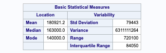
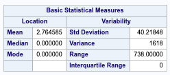
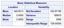
Sales price – Since we are seeing a very large range within our housing price data, we will need to perform a log transform of the sales price when making our predictions, and then back transforming when we submit to kaggle. The goal here is to stabilize the variance and reduce the effect of outliers within our dataset.

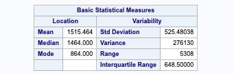
Gross Living Area – Due to the large variance in the gross living area, we will need to enact a log transform in our study.

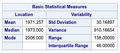
Lot Area – Since our variance in lot area is very large, we will need to run a log transform. Als due to the difference in mean and median, we can assume that this data is slightly left-skewed.

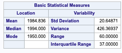
Year built – among our data set, the average age of houses in Ames Iowa is a little under 40 years old, with a median age since remodeling is 14 years.

The 2nd Floor Square footage and the presence of a swimming pool may ultimately play a role in the price of a house due to the implication of a larger house having two stories.

Analysis 1

Restatement of Problem  

Our goal with the assignment is to measure the relationship of the Sales Price and Gross Living Area of a house and how that can be affected by the Neighborhood a house is located in. For this particular analysis, we will be focusing on just the North Ames, Edwards and Brookside Neighborhoods. In particular, we will be working towards conducting a hypothesis test of our null, which that there is no difference between the sales price and gross living area of our houses between neighborhoods, and our alt hypothesis that there is a significant relationship between the neighborhoods.

Build and Fit the Model

Log of sales price = B0 + B1(logsqft)x + B2(NAmes) + B3 (Edwards)

This means that to predict the log of the sales price of a Brookside home based on the square footage, we would start at a y-intercept with a slope determined by the square footage. For the North Ames and Edward neighborhoods, the y-intercept value will decrease or increase based on the estimation variables we will determine later on.

Checking Assumptions

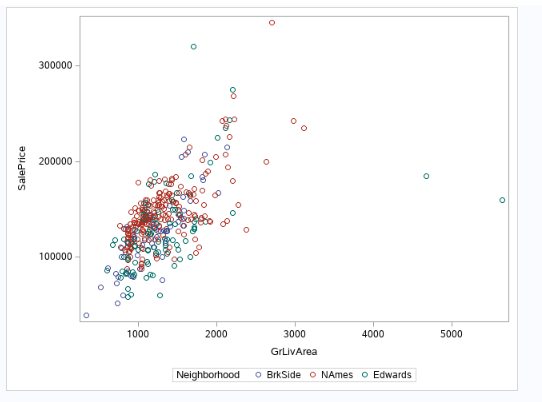
Figure 0-1 (scatter plot of gross living area, sales price colored by our 3 neighborhoods)

Here’s a quick scatter of sales price and Gross living area across our 3 neighborhoods within the raw data. We can see that we can potentially see a higher sales price of the North Ames compared to the Edwards region due to the higher the red is in relation to the green, but we will need to do further testing. Additionally, a log-transform may help clearly convey our message.

Looking at the residual plots (fig 0-2) to help check assumptions, there is no evidence against normality of the log of the sales prices, as well as the log of the gross living area Viewing our scatters and leverage plots, there is no evidence against constant variance of log of sales prices across our living area. Based on our scatter plots, we can also see no evidence against a linear trend between the sales price and living area. For this particular study, we will assume the Sales Prices are relatively independent and that our selection procedure solved the multicollinearity issue. Looking at the Cooks D, we can see that there are a couple of high leverage points that we will need to address.

Figure 0-2 (log transform of our square footage and sales price in relation to neighborhood, along with the other diagnostic residual plots to assess assumptions)

Looking at the separate regression lines for the 3 neighborhoods (figure 0-2) we can see the that North Ames has a slightly higher intercept than with Edwards and Brookside, which could potentially infer that the price per square foot is higher than that particular neighborhood than the others. With that said, we can see there are a few outliers that could potentially garner a lot of leverage, but let’s review.  

We ran a VIF measure of a model including the log of our square footage with its interaction terms relating to each neighborhood. As you can see we are seeing extremely high VIF values, which is the measure of collinearity of each predictor variable in the models (i.e. the effect of multiple values affecting the Generally, if our VIF exceeds 10, then you can expect major problems, so it’s concerning that we are seeing VIFs over 800.

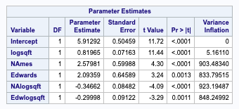
Figure 0-3 (Cook’s D and VIF of our log of square footage, price and the neighborhood. Note how the variance inflation is at 800-900, which is massively overly collinear)

Removing the interaction terms, we can see that the Tolerance values (Variance inflation) are much lower and within 1, which indicates we have little collinearity (aka. Two variables in our model impact the sale price in the same way).

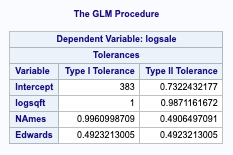
Figure 0-4 (tolerance measure of our variables. Since they are below 1, we can infer there is little collinearity.

From an initial analysis for influential points in the log-log model, the observations that really stand out are

146, 22, 91.  Obs 146 and 91 are highly influential given their large leverage and high studentized residual values.  These are unusually spacious residencies in the Edwards neighborhood. This can be observed in the scatterplot below.  Since these residencies seem to be non-representative of the overall Edwards neighborhood, they will be removed. The model’s R2 somewhat improves, but observation 22 still stands out.

With that said, our Cook’s D plot is showing that there are still a few values that are showing a few influential variables, including 146 and 91, which we can explore removing as a possibility to make our model more efficient and predictive.

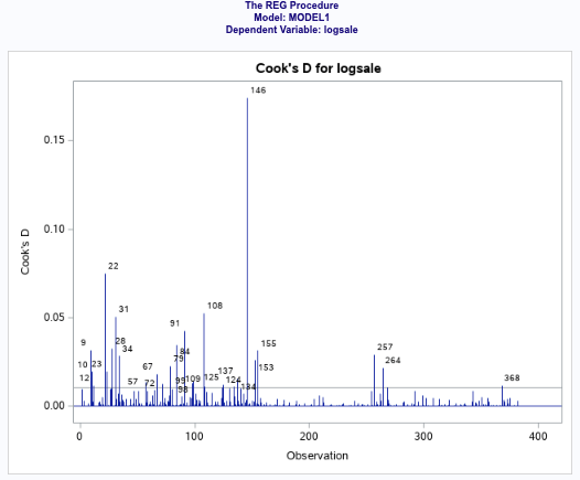
Figure 0-5 (cook’s D of our influential variables. )

After rerunning our model (model 5) with without the 146 and 91 values, our tolerance values did not change, but we were able to see our standard errors were minimized. Despite having high leverage, removing this observation does not significantly change the regression coefficients of the model so it will be kept in the model since it’s not influential.  

Reviewing the new Cooks D chart for model 5 (figure 0-6 – in appendix), the only remaining problematic values is 22. We can rerun the model to see if the results change much.

After doing so, we can see that the model doesn’t change much, and the R2 is starting to drop. So we can leave the 22 value in for our analysis. In addition, we are seeing the adjusted R2 dropping from 50% to 47.8%. Furthermore, Cook’s D is less than 1 for the remaining observations so they don’t need further investigation.

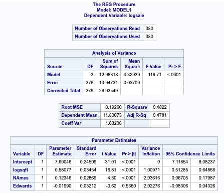
Figure 0-7 (coefficient data for our model 4)

Model 5: Adj R-Square (0.4822)

Model 4: R – Square (0.50)

Moving forward, we will use the house 4 model to fit our regression equation.

 

Parameters

Reviewing the GLM procedure of our winning estimation model (figure 0-8 – in appendix), we are able to ascertain that the log of the sale price of Brookside will have an intercept of 7.48 with the North Ames Neighborhood accounting for an increase in 0.13 in the intercept of the sale price, while Edwards will have a -0.01 decrease in the intercept. This is consistent with figure 0-2 which supports the conclusion that Edwards has a significantly higher Sales Price in relation to square footage among the set of 3 neighborhoods.

logSalesPrice(hat) = 7.48 + 0.60 (logsqft) + 0.13(NAmes)  – 0.01 (Edwards)

The individual regression equations are below.

Brookside: (where Edwards and NAmes = 0

LogSalesprice (hat) = 7.49 + 0.60 (logsquarefoot)

 

Edwards:(where Edwards = 1)

LogSalesprice (hat) = 7.49 + 0.60 (logsquarefoot) -0.01 (Edwards)

 

NAmes: (where NAmes = 1)

LogSalesprice (hat) = 7.49 + 0.60 (logsquarefoot) + 0.13(NAmes)

 

95% confidence intervals

Figure 0-8 (covariance of estimates – we will use this covariance to build our confidence variables against our critical value of 1.97)

Var(NAmes – Edwards) = 0.0008 + 0.00103 – (2* 0.0006)

SD(NAmes – Edwards) = 0.00183 – (0.0012) =  0.00063

 

Critical value (0.0975, 378) = 1.97 * 0.00063 = 0.0012

95% CI (NAmes): 0.13 +- 0.0012 = (0.01, 0.25).

95% CI (Edwards): -0.01 +- 0.0012 = (-0.0112, -0.0088).

 

Statistical Conclusion

Reviewing the individual regression equations for the 3 neighborhoods, we are seeing there is a significant difference (p-value of <0.001)in the intercept of the NAmes regression line compared to the BrkSide regression line. This is not the case with the Edwards line with the p-value of 0.66.

 

Analysis 2

 

Restatement of Problem  

A common challenge with real estate firms is to determine the returns they can expect on their investments and how much to invest in their home inventory. With homes having so many features to compare against, how do you predict the market value for a home? We are going to look at some real estate data from Iowa of over 1,400 homes with 81 defining features, and run 4 different prediction models to see if we can determine what price a home is going to fetch on the market.

Forward Selection

Forward selection is a traditional model selection procedure that sequentially adds in new variables to a model unless their inclusion does not add a significant improvement to the effect. In this case, our response variable is the log of SalePrice and our forward selection sequentially worked through our list of 80 variables, adding new predictors until the F statistic no longer improved.  All explanatory variables are initially coded into the model, the model worked under the assumption that NA’s were relevant data and the model would weed out irrelevant NA’s not reflective of missing data, which is an assumption that would carry over across all our models.

Checking Assumptions

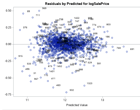
Fig. 1-1 (residual plot of the log sale price)

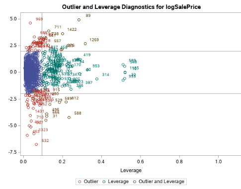
Fig. 1-2 (leverage diagnostics for log sale price)

 

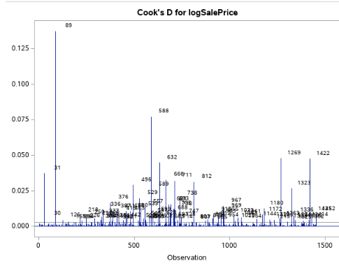
Fig. 1-3 (Cook’s d)

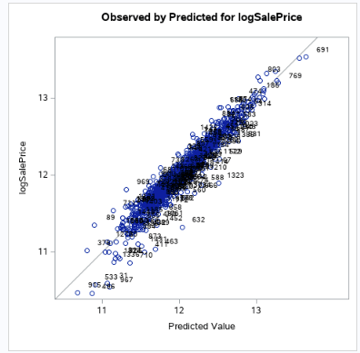
Fig. 1-4 (Actual (log) vs Predicted)

Looking at the residual plots (fig 1-2) to help check assumptions, there is no evidence against the normality of the log of the sales prices, as well as with the 20 variables we came out with. Viewing our scatters (fig 1-4) and leverage plots, there is no evidence against constant variance of log of sales prices across our variables. Based on our scatter plots, we can also see no evidence against a linear trend between the sales price and our variables. For this particular study, we will assume the Sales Prices are relatively independent and that our selection procedure solved the multicollinearity issue.

Looking at figure 1-3, observation 89 appears to be a bit troublesome so we can remove to see how it affects our Cook’s D. In figure 1-5, you can see that removing it will help curtail the influence a single value can have on the model.

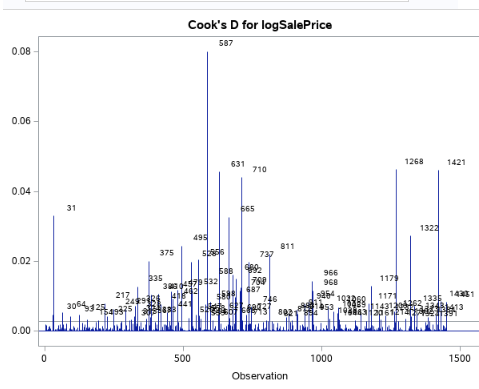
Fig 1-5 (Cook’s D – with obs 89 removed)

 

Model Performance Metrics

After applying our data transformations to the testing data set that we used for the training set, which included changing the character type for Lot Frontage as well as the log transforms to the sale price, we were able to run a proc glm procedure to calculate the CLI prediction for our sales price using the data from the first 1400 housing metrics.

In doing so, we were able to generate an R2 value of 0.9324, which essentially means that over 93% of the variability of the median (note we had to take a log transform and back transform our result) housing prices can be explained by the model we chose. This means, that 93% of a housing price score can be predicted by factors such as Lot Area, Land Slope, Neighborhood, home condition, building type, Roof Material, etc (full list below). Running the data through Kaggle, we received a root mean square error of 0.26 which calls out how far our data falls from our regression line of predictability. On a scale from 0 to 1, this means the model is weak in its ability to predict, which is expected with a Forward selection. Our model also provided a press statistic of 16.43 against the observations that were not used in the training model to generate the score.

(Final Performance figures can be found in the appendix)

Backward Selection

Similar to the forward selection, the backward selection is also a traditional model selection procedure. However, the key difference is that with a backward selection procedure, the model starts with all 80 variables and sequentially removes variables until a stopping condition is satisfied. In this case, our response variable is the log of SalePrice and our backward selection sequentially worked through our list of 80 variables, removing predictors that did not have a major effect on the F value.  All explanatory variables are initially coded into the model, the model worked under the assumption that NA’s were relevant data and the model would weed out irrelevant NA’s not reflective of missing data, which is an assumption that would carry over across all our models. Our backward procedure determined the following variables will be most predictive.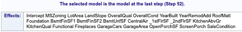

Fig 2-1 (list of predictors that our Backwards procedure selected)

Checking Assumptions

We ran the same data cleaning methods that were used in the forward selection to ensure consistency in the comparison of our models.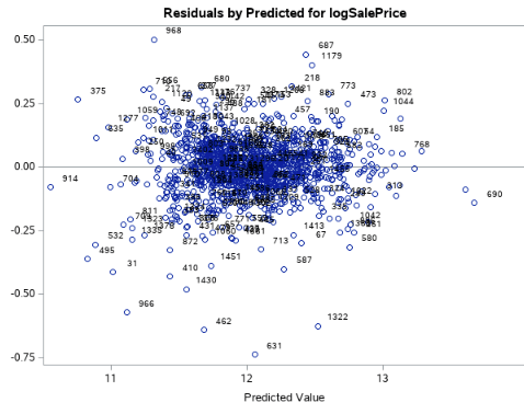

Fig 2-2 (Residual plot of the log sale price)

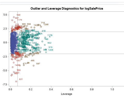
Fig 2-3 (Leverage and outlier diagnostic of the log sale price)

 

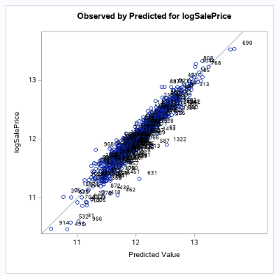
Fig 2-4 [Left] (Observed Scatter plot of sales price)

Fig 2-5 [Right] (Leverage and outlier diagnostic of the log sale price)

Looking at the residual plots (Fig 2-2) to help check assumptions, there is no evidence against the normality of the log of the sales prices, as well as with the 47 variables we came out with. Viewing our scatters (Fig 2-4) and leverage plots (Fig 2-5), there is no evidence against constant variance of log of sales prices across our variables. Based on our scatter plots, we can also see no evidence against a linear trend between the sales price and our variables. For this particular study, we will assume the Sales Prices are relatively independent and that our selection procedure solved the multicollinearity issue.

Model Performance Metrics

After applying our data transformations to the testing data set that we used for the training set, which included changing the character type for Lot Frontage, removing the problem data from our Cook’s D plots as well as the log transforms to the sale price, we were able to run a proc glm procedure to calculate the CLI prediction for our sales price using the data from the first 1400 housing metrics.

In doing so, we were able to generate an R2 value of 0.9299, which essentially means that nearly 93% of the variability of the housing prices can be explained by the model we chose. This means, that 93% of the median housing price score can be predicted by factors such as Lot Area, Land Slope, Neighborhood, home condition, building type, Roof Material, etc (full list in fig 2-1), which is also very similar to our forward selection procedure. Running the data through Kaggle, we received a root mean square error of 0.26 which calls out how far our data falls from our regression line of predictability. On a scale from 0 to 1, this means the model is weak in its ability to predict, which is expected with a Forward selection. Our model also provided a press statistic of 16.77 against the observations that were not used in the training model to generate the score.  All in all, the backward selection procedure performed very similarly to our forward selection procedure in our key metrics, which would suggest that there was a major drop off in predictability within a core group of variables in our dataset as compared to the others.

 

Let’s see how we performed in the stepwise and custom models to see if more can be learned.

Stepwise Selection

Stepwise selection can be considered a hybrid between Forwards and Backwards selection.  In this case, our response variable is the log of SalePrice.  All explanatory variables are initially coded into the model, trusting that it will weed out variables with majority NA values (and it does, as will be seen later).  

Checking Assumptions

Residuals

           

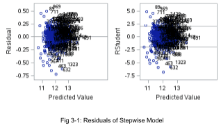
From Figure 3-1 the residuals (both regular and studentized) tend to follow a random cloud pattern around 0.  There are no dramatic departures from normality, and with such a large sample size the model is robust to moderate non-normality.

Influential Point Analysis

In a combination of Figure 3-1 and 3-3, there’s no reason to believe any points are unduly influential.  With a large dataset, it’s unsurprising that ~ 5% of data points fall outside two standard deviations from the mean. Furthermore, no point features Cook’s D > 1.  Even the cluster of points with leverage between 0.6 and 0.8 have studentized residuals within 2 sd. As a result, we have little reason to investigate any other observations that the two observations (524 and 826, see Fig 3-3) are accounted for in the final Stepwise model.  Fig 3-4 shows the final model with those two observations removed. 

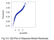
That being said, it is possible to further log transforms can alleviate the slight departure from normality, and this can be examined in later research.

Model Performance Metrics

The variables included in the model are in Figure 3-5, with 22 predictor variables out of 81 original variables.

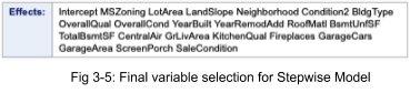
The adjusted R2 evaluates to .9226, which means that ~ 92% of the variation in median Ames sales data is explained by this stepwise model.  The Kaggle score is .133, which is pretty low considering the relative simplicity of regression versus more advanced techniques like boosting and ridge regression.  The PRESS Statistic is 19.67.

Custom Model: Forward Selection with 10-Fold Cross-Validation

The final model to evaluate will be a modification of the Forward Selection model described earlier.  As before, the response will be logSalePrice.

Checking Assumptions

Residual Plots

As a first-pass model, we can see two houses are highly influential, obs 1299 and 524.  These two houses have abnormally high LotArea values.  So we will remove these and rerun the revised model.  Figures 4-1 and 4-2 show the before and after, and the latter is much better.  As before, it’s not unusual to have a large dataset with ~5% of data points outside 2 sd.

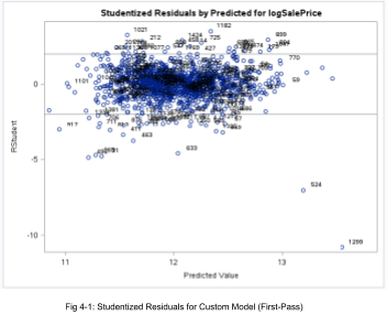
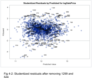
Furthermore, Fig 4-3 suggests no drastic departures of normality in the revised model.

From here forward, any analysis we will be referring to this revised model.

Influential Point Analysis

We might be afraid at first of the two observations in Fig 4-4 with high leverage, but the studentized residuals are near 0.  In Fig 4-5, all of the Cook’s D values are very small, so Figures 4-2 and 4-5 imply no reason to worry about influential points.

Model Performance Metrics

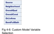
The final iteration of the cross-validation yields the following variables (Fig 4-6).  The beauty of this model is the variables make intuitive sense and retains only 5 of 81 observations with an R2 of .86 on the test set.  This means almost 90% of the variation in the median sale price is explained by just these 5 variables.  The CV Press comes out to 32.95 and a Kaggle score of .1556.

Comparing Competing Models

It is interesting that Forward Selection produces the highest R2 and lowest CV Press, but the least-performing Kaggle model, relative to the other three models.  However, the Stepwise model has the lowest (best) Kaggle score amongst the four models, which implies it has the best predictive power.  A summary of the performance metrics can be found in Fig 5-1.

 

Model	Adj R2	CV Press	Kaggle Score
Forward	0.9324	16.44	0.26
Backward	0.9299	16.77	0.26
Stepwise	0.9226	19.67	0.133
Custom (Forward Selection w/ 10 Fold Cross Validation)	0.86	32.95	0.1556

Fig 5-1: Comparison of Model Performance Metrics

Conclusion

After tweaking the data set to omit data and columns that were overly influential to our regression model, we were successful in implementing four unique regression modeling techniques to accurately predict sales prices in Ames, Iowa.  Overall, our stepwise procedure garnered the strongest Kaggle Score (Root mean square error) with our forward selection driving the strongest R^2. It proves one doesn’t need fancy deep learning models to achieve commendable results. For further study beyond the scope of this course, we would love the opportunity to apply more robust data since procedures like a random forest to see how our Root Mean Squared Error could possibly improve.

 

In November, I rode a Citibike around midtown. Then a week later, I used Citibike’s open data to see if I could use the data to figure out where the bike was after a week.

CitiBike Project

I was able to extract a lot of event data from Mozilla Firefox to see how people use bookmarks and tabs in their browsing. I was tasked to make a recommendation on whether we should focus on optimizing the tabs or the bookmarks in the upcoming version update.

Mozilla Firefox presentation

Outbrain Presentationfrom (1)

 

Continue reading →

For the first week of October 2014, I had the opportunity to spend a week in Thessaloniki, Greece. Below are photos from the week.

Continue reading →

Unlike your typical adolescent boy, I had often found myself fantasizing about being a sports announcer. Unlike the other kids at school, who wanted to become monster truck drivers and lawyers, my childhood dream job was to go to exotic locales(with professional football franchises) on a weekly basis and spending the better part of 3 hours giving play-by-play about the off-field story lines and how it leads to the on-field drama. My moist-laden microphone would have been my Rosebud and Howard Cosell was my Citizen Kane.

But sadly, my dream of being the voice of a new NFL generation died as soon as I heard the sound of my own voice mail message when I was programming my first cell phone. It was the moment I learned I could possibly have an effeminate voice. This was all happening when I was sixteen years old and still going through puberty, but the shock managed to last.

While reality slipped away in the years that followed, I still found myself thinking the “what if’ thoughts. What if I had rocked my high pitched squeal as a normal speaking voice? What if I had enrolled in the Sports Broadcasting classes in high school? What if I had pressured my mom into buying me a blazer at a younger age?

In the midst of all this self-questioning, I was able to find at least one answer. Fortunately, for my outlandish world where I decided to follow my dreams in life, it was the most important answer. The one that would have defined my career as a Sports broadcaster and would have forged my name in the stone only reserved for the greatest legends of the game. It was what my signature line would be. It was “Backdoor Charlie”.

What is a “Backdoor Charlie” you ask? ‘What isn’t a “Backdoor Charlie?”‘ would be my response with a question to that question. To give visual representation, see this video for a list of the top 10 plays in week 4 of the 2014 NFL season. Of the highlights listed, about 7 of which are certified “Backdoor Charlies” according to myself.

It would have been perfect. Week in and week out, I would narrate the plays unfold as days of preparation manifested itself into a 3 hour exhibition of strength, strategy and speed. On the rare occasions when all three aligned in harmony(or didn’t), “Backdoor Charlie” happened. Whenever people would have asked me what a Backdoor Charlie was, my response would have been incredibly vague and I would have used it at completely random times.

“Peyton Manning fakes the hand off and delivers a Backdoor Charlie to Julius Thomas.”
“Cameron Wake explodes off the snap, puts the right tackles into a Backdoor Charlie and sacks Tom Brady.”
“THE BAND HAS BACKDOOR CHARLIED OUT ONTO THE FIELD. HE’S GOING TO GO INTO THE END ZONE. THE BEARS SCORE!”
“Christian Ponder threw a Backdoor Charlie that was intercepted by Clay Matthews.”
“Jake Locker scrambles from the pressure, and does a Backdoor Charlie to his left knee. And now he’s not getting up.”

It would have been a long con, but nothing should come easy. Not even in your own fantasies.

OBJECTIVE: Revive Kleenex from mediocrity into the spiritual force a tissue brand could be.

CHALLENGE: Due to its monopoly of success across the globe, Kleenex risks it’s brand name becoming the generic catch-all name for the category and subject to losing it’s trademark.

In addition, Japanese consumers do not know the difference between the quality of Kleenex tissue and it’s inferior competitor, Puffs.

TRUTH: As the nation of Japan rebuilt itself from World War 2 in the latter half of the 20th century, government officials and Buddhist monks launched an experimental genetic program that would breed an army of grass ogres with the power of divine touch on all objects they came across. The secret program was called Hiiragibusshu ikimono and it would pave way for Japan’s dominance in the technological revolution. Wanting a piece of the magic, Kimberly-Clark CEO Darwin Smith, called upon these grass ogres to bless their brand of tissues with a softness, lightness and freshness that no other tissue has ever seen before. All for a substantial donation to the program.

ANSWER: Kleenex tissues have the power to not only wipe your snotty nose with a power an efficiency never seen before, but transcend into shaping a greater good.

PROOF: While the particulars of Hiiragibusshu ikimono are heavily classified, the grass ogres have left the tissues 10% lighter and 4% softer than any competitor’s tissue. Also, in qualitative product research, participants noted greater feelings of euphoria when using the product.

RESULT: Link

My great-great-great grandpa, Otto Paulsen, grew up as a hippie in the late 1800 Scandinavia. While other folks of his time parlayed a rigorous work ethic into a life of honest success, He spent much of his time empathizing with Nordic woodland creatures and embellishing facts about himself to impressionable kids. While admiration was hard to come by within his persona, one would fain to ignore his inability to live life by any other means in his own terms. For this reason, authority saw him as a barrier to the way things should be. Working at (what I would assume) was something related to the fishing industry, he was constantly tardy and insubordinate with simple company policy. Otto was not wired for European life so he set sail to America with only the clothes on his back and a bindle of peyote he traded his money and supplies for. His notorious Swedish ways were not left at home as he theived his way into sustainability, all the way to stealing the identity of an unsuspecting nephew of an oil tycoon, Doug Clark. However, one day he fell in love with a German maiden named Denise and settled his miscreant life down in order to convince her he wasn’t too creepy to marry.

Natural selection took hold and I was born 100 years later.