Introduction

With the NFL pushing nearly $8.2 billion in revenue in 2017, the league is becoming bigger business than ever before. With more at stake for teams to be successful, there is a massive emphasis placed in scouting college athletes and finding those with the greatest aptitude towards performance in a professional football setting. 

 

This is not an exact science by any measure. For all the many success stories of diamonds being selected in the rough to go on to have great careers in the NFL, there have been some famous missteps by teams investing their future into a new player who ultimately did not pan out. Fans of the NFL have a not so delicate way of referring to these players as “busts.”

 

The flagship event in the scouting process in professional football is what is called the NFL Combine. This 3 day long event typically held in Indianapolis, IN, is a gathering of all the top athletes in college football to demonstrate their strength, speed, agility while also getting their official heights and weight data for teams to analyze when making their selections for the next year. 

 

One of the most popular events at the combine is a 40 yard dash, known as the “Forty”. The reason why it is most popular at these events is not only because it’s exciting to see these athletes running 25 mph across a football field, but it also is considered to be one of the most reliable measures of future performance in the scouting process. The logic makes sense, as you can teach technique and strength all you want within a player, but if they can’t get from A to B faster than the other guy, then they are not going to be able to make a play. 

 

For this project, we are going to review about 17 years of combine data (dating back to the year 2000 when electronic timing for the Forty was implemented, and see if we can detect patterns within player attributes to figure out what would generate the fastest 40 time among prospects. 

 

Data Description and Overview

 

Data Overview

The dataset includes a population of over 6,000 NFL draft prospects that appeared and tested in the combine from 2000 to 2017 with 15 explanatory variables describing some detail about the players, including position, height and weight as well as some of the combine performance data including how many reps they could bench press 225 pounds, vertical jump, broad jump and the shuttle drill. The data came from Kaggle and includes the 40 times for the players which range from 4.24 (the fastest time ever recorded) to 6.05 (the slowest time ever recorded). The goal of the assignment is to see if we can take some of the other explanatory variables to predict the forty time of each player. Including the 40 time, below is an explanation of some of the other variables involved in the study.

 

Combine results reported in this study Include 

• 40-yard dash 
  • The 40-yard dash is a test of speed and explosion. Starting from a three-point stance, the player runs 40 yards as fast as possible. Times are recorded in 10-, 20-, and 40-yard increments.  
• Bench press 
  • The player’s goal in this exercise is to bench press 225 lb as many times as possible. With the exception of quarterbacks and wide receivers, all players participate in this test of upper body strength. 
• Vertical jump 
  • To measure the vertical jump, a player stands flat-footed in front of a pole with a number of plastic flags sticking out. The player then jumps from a standing position and swats as many flags as he can, thus enabling the judge to determine how high the player can jump. This exercise is considered important for wide receivers and defensive backs, where jumping ability is a critical skill. 
• Broad jump 
  • The broad jump measures how far a player can jump from a standing position. This drill is most important to positions that use lower-body strength (such as offensive and defensive linemen) to gain an advantage. 
• Cone drill 
  • In this exercise, three cones are set up in a triangle shape with each cone 5 yards apart. Starting in a three-point stance, the player sprints in a predetermined route among the cones. This exercise tests speed, agility, and cutting ability. 
• Shuttle 
  • In this exercise, the player starts in a three-point stance and runs 5 yards in one direction, 10 yards in the opposite direction, and then sprints back to the starting point This exercise tests lateral speed and coordination. 

 

Population of Interest

The population of interest in our study are the 6000 participants in the NFL combine. These participants are former college athletes from the United States with a great skew towards athletes who played varsity football in college. Per the NFL rules, the athletes need to be at least 3 years out of high school, so the majority of the data is from athletes who are ages 20 and over. 

 

There is also an invitation process for college athletes, so the best of the best players in the NCAA are only invited to the combine. Out of over 10,000 players active in the NCAA, only 335 are invited to the combine each year. 

 

EDA

Looking at our key response variable in our data set, the forty time, we can see that there is a small variance between 40 times with 75% of the data being below 5 seconds (which is much faster than you or I could run). We can see the mean 40 time is 4.78 with a median of 4.70, which would suggest there is a right skewness to our data.

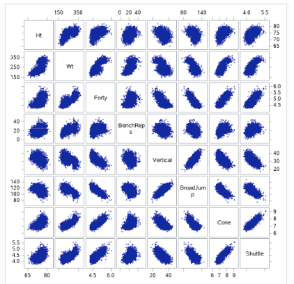
Fig 0-1 (workout scatter plots)

 

Looking at the combine performance data, we can see some clear positive/negative relationships happening between players who perform well in some events and their performance on others. For example, we can see that players who have a lower 40 times tend to not be able to bench press as many times, and we can see that faster players do not seem to jump as high or as long. Which may be related to height, it appears that shorter players are faster, per the scatter.

 

In Fig 0-2, we can see the 40 time by position group. Here, we can see that the faster positions in the NFL are DB, WR, S and CB, while the slower positions are offensive linemen (who are known for being bigger players) such as Centers, Guards and Tackles. 

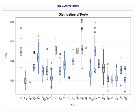
Fig 0-2: Analysis of Variance between positions

 

Looking at an analysis of variance between position and 40 time (fig 0-3), we can see the distinction between positional roles on a team and how fast the players can run. Offensive linemen positions (OG, OT, G, C) as well as the defensive nose tackle position all tend to have slower 40 times with means of 5.25. While slower, this makes sense because these types of positions tend to favor power over the other positions, which focus on speed and separation. The faster positions we tend to see are Cornerbacks (CBs), Safety’s (S), Running Backs (RBs) and Wide Receivers (WRs) with a mean forty time of just over 4.5. 

 

Analysis  

 

Restatement of Problem  

 

The primary purpose of this study is to examine some of the measures that are part of the NFL combine each year and see how they can go to predict the 40 yard dash time, which is considered to be the flagship measure of a player’s capability in the NFL. This will notably include the performance measures of non running events as well as positional attributes within the players. As we see in fig 0-1, 40-yard dash ( forty) has a linear positive relationship with weight, height, bench press, cone drill, and shuttle. In addition, it has a strong negative linear correlation with Vertical jump and Broad jump.  As we see in fig 1-0 and 1-1, there are some outliers or leverage or both, but one observation has high in magnitude. 

 

Build and Fit the Model 

 

Forty= 𝛽0 + 𝛽1Wt + 𝛽2Ht + 𝛽3BenchReps+ 𝛽4Vertical  + 𝛽5BroadJump + 𝛽6Cone + 𝛽7Shuttle 

 

Checking Assumptions

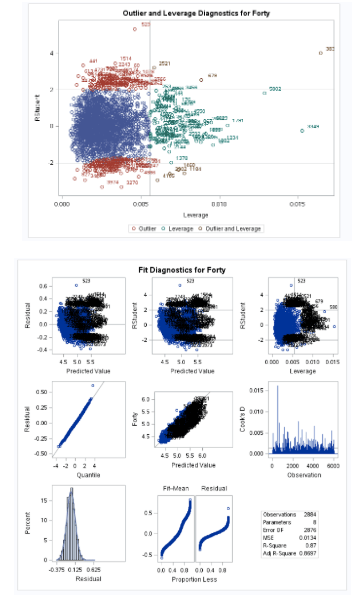
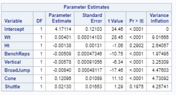
Fig 1-0: Outlier and Leverage diagnostics

Fig 1-1: Residual plots and diagnostics

In figure 1-0, we can see observation 3878 is a high leverage point with regards to 40 time. Doing some research, we can see this observation is of Isaiah Thompson, who is known for having the slowest 40 time in the history of the combine at 6.04 seconds. Using an NFL analyst, Rich Eisen forty time of 5.97 as a control time (since he was 48 years old and wearing a suit), we can use this as cause for dropping Isaiah Thompson’s time due to his performance being not up to the standard of performance that a player would need to be at to be someone who was invited to the combine.

After dropping Isaiah’s time, we can see that our regression model better meets the assumptions that we would need to satisfy our regression model, even without transformation needed to our dataset.

Normality – reviewing the histogram plot available to us, we can see that while there is a slight right skew. However, it doesn’t seem significant enough to warrant us applying a transformation to our data.  This right skew is natural since it is much easier to get a slower 40 time than it is to get a sub 4.3 forty.

Constant Variance – regards to constant variance, we can see through our residual analysis that we have a pretty consistent cloud at the low values and a little more scattered at a higher value. However, after trying a transformation of a log of the 40 time, we cannot see a significant improvement. 

Linear Trend – The linear trend analysis shows all the data fits pretty cleanly on a single regression line. 

Independence – While the fact that many of the players in the combine have the same coaches, which may have a covariate effect on scores, it doesn’t seem significant effect to be troublesome in our analysis. So we will assume independence moving forward. 

 

Looking at the Variance inflation factor in Figure 1-1, we are not seeing any evidence of collinearity between the factors we will use for our study. Typically, we would be concerned if we see any VIF scores at above 10 for a variable. 

 

Model Performance Metrics

All explanatory variables are initially coded into the model, the model worked under the assumption that NA’s were relevant data and the model would weed out irrelevant NA’s not reflective of missing data, which is an assumption that would carry over across all our models.

After going through the model assumption and model assessment we come to the model selection. Using the dataset, we would like to explore the factors that contribute to a good performance in the response variable ( Forty). We will attempt to create a predictive model to accurately predict the response variable Forty using multiple selection methods, including stepwise selection, LASSO and LAR model.

In the variable selection process and fit diagnostics we haven’t done any variable transformation as conformity to linear regression model is achieved through multiple benchmarks stated in the previous sub chapters.

To filter the best candidate regressing variables we used GLMSELECT procedure cross validation was used as our selection criteria, with no stop criteria. Cross validation is a more effective significance measure because of how it “leaves out” observations as they are examined, to validate the significance of variables at each validation.

Below is a table outlining some of the performance measures of the model selection methods that we used

Predictive Models Adjusted R Square CV PRESS

Stepwise .86 38.65

LASSO .86 38.66

LARS .86 38.66

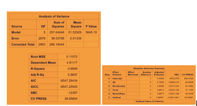
Fig 2-1: Stepwise Regression Technique with CV stop (leaves shuttle out of our final model)

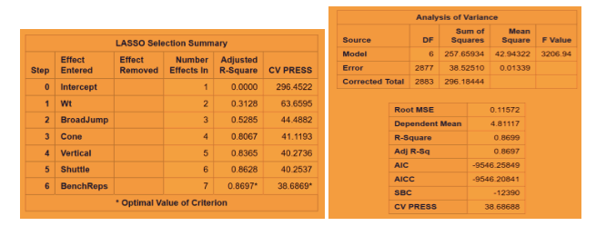
Fig 2-2: LASSO regression technique with CV stop

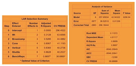
Fig 2-3: LAR regression technique with CV Stop

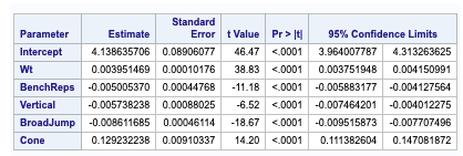
Fig 2-4: Confidence limits for LAR and LASSO

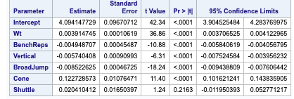
Fig 2-5 Confidence Limits for Shuttle

 

The minimum CV press value for the forward selection is given Dependent mean is the mean of the response variable. The Adjusted R Square (Coefficient of determination) and R square values are the degree of measurement of how the response variability is explained to the predicting variables ranging from 0 to 1 where the closer to one the better for adjusted R. The mean Squared Error ( MSE) : For prediction is simply the average of the squared deviations between the Fitted values and the observed data. In our model selection run down the three model selection show pretty much similar RMSE. I used CV press as a model KPI because Cross validation though It is error criterion not selection criteria but it’s helpful when paired with Selection criterion breaking the data into training data set and test data set to get a more accurate assessment of the predictive accuracy of a model. Other selection criterion AIC ( Akaike’s information criterion) which denotes how well the model ( log likelihood) plus how complex the model ( penalizes the model fit by the number of regressors is also displayed for all the three section techniques. BIC ( Bayesian Information criterion) also called SBC is part of the descriptive statistics. For our comparison we choose adjusted R square paired with cv press as a good indicator to pick the best selection model as shown above in the table. Looking at the confidence limits for LAR and LASSO model as well as the Stepwise model, we can see that the addition of the Shuttle Drill would make a marginal change to the linear regression line. 

 

The final Model (custom model)

The best candidate predictors that dictate how well the response variable is regressed by the candidate or indicative variable is fitted below with corresponding coefficients in linear fashion.

How the 40-yard dash ( test of player speed and explosion ) is regressed by the prediction variables like weight of the player , Bench press( count of bench pressing 225lb) , height of vertical jump , Broad Jump( how far player jump from standing pose) , cone drill ( as a measure of player agility )

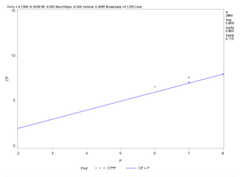
Fig 2-4 Regression Procedure

Conclusion

After tweaking the dataset to remove an outlier time for forty (which we justified due to the player performance not being considered up to standard with the athletes that are typically invited), we have been able to successfully build a regression model that can predict Forty time performance based on the performance of other events at the combine. 

 

After implementing thress regression modeling techniques (Stepwise, LAR, LASSO), we were able to garner successful model fitting with an adjusted R^2 value of 0.8697 and a Root Mean Square Error of 0.115, which is strong enough to show success of the predictive ability without being overfit to new data. This was support using cross validation stopping techniques when running the model selection procedure. 

 

With all that said, we would consider selecting the Stepwise selection procedure as the strongest model because it is able to achieve the same R^2 and RMSE value while using less variables and it’s AIC value is slightly lower. 

 

For further study beyond the scope of this course, we would love the opportunity to access some of the data from the player’s performance from college to predict a player’s 40 time, and potentially use that information to predict future player 40 times based on their college performance data. If this becomes reliable, the NFL can save millions of dollars in resources to assess player performance across the college landscape without the costs to hold events to have players run the 40.